4.6 Quantifying equate fit

It is essential to activate only those equate groups for which the assumption of equivalent measurement holds. We have already seen the item fit and person fit diagnostics of the Rasch model. This section describes a similar measure for the quality of an active equate group.

4.6.1 Equate fit

Section 6 of Chapter I defines the observed response of person \(n\) on item \(i\) as \(x_{ni}\). The accompanying standardized residual \(z_{ni}\) is the difference between \(x_{ni}\) and the expected response \(P_{ni}\), divided by the expected binomial standard deviation,

\[z_{ni} = \frac{x_{ni}-P_{ni}}{\sqrt{W_{ni}}},\]

with variances \(W_{ni} = P_{ni}(1-P_{ni})\).

Equate infit is an extension of item infit that takes an aggregate over all items \(i\) in active equate group \(q\), i.e.,

\[\mathrm{Equate\ infit} = \frac{\sum_{i\in q}\sum_{n}^N (x_{ni}-P_{ni})^2}{\sum_{i\in q}\sum_n^N W_{ni}}.\]

Likewise, we calculate Equate outfit of group \(q\) as

\[\mathrm{Equate\ outfit} = \frac{\sum_{i\in q}\sum_{n}^{N_i} z_{ni}^2}{\sum_{i\in q} N_i},\]

where \(N_i\) is the total number of responses observed on item \(i\). The interpretation of these diagnostics is the same as for item infit and item outfit.

Note that these definitions implicitly assume that the expected response \(P_{ni}\) is calculated under a model in which all items in equate group \(q\) have the same difficulty. This is not true for passive equate groups. Of course, no one can stop us from calculating the above equate fit statistics for passive groups, but such estimates would ignore the between-item variation in difficulties, and hence gives a too optimistic estimate of quality. The bottom line is: The interpretation of the equate fit statistics should be restricted to active equate groups only.

4.6.2 Examples of well fitting equate groups

The evaluation of equate fit involves comparing the observed probabilities of endorsing the items in the equate group to the estimated probability of endorsing the items in the equate group. For an equate group there is an empirical curve for each item in the equate group and one shared estimated curve. The empirical curves should all be close together, and close to the estimated curve for a good equate fit.

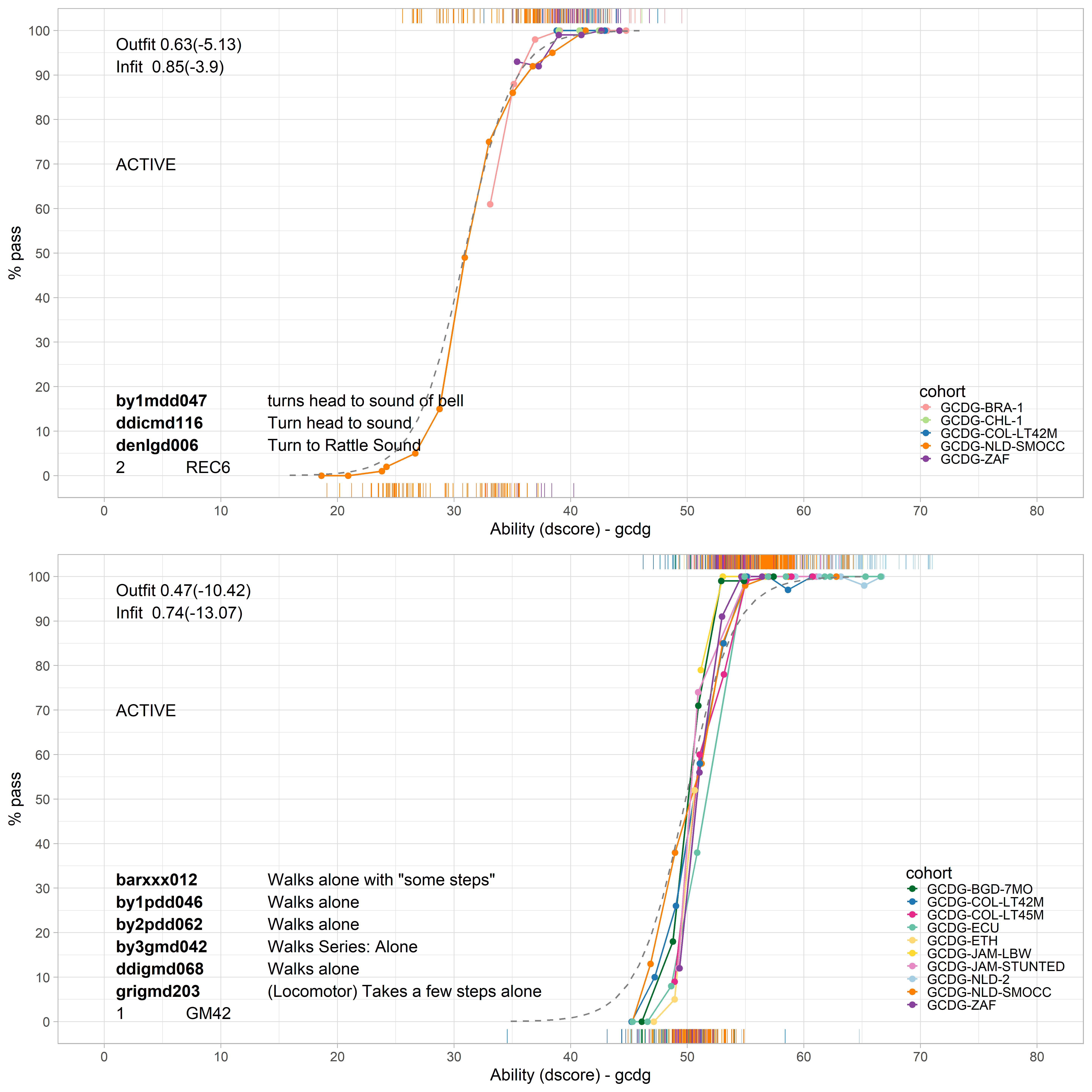
Figure 4.4: Two equate groups that present a good equate fit.

Figure 4.4 shows a diagnostic plot for equate groups REC6 (Turns head to sound of bell) and GM42 (Walks alone). The items within REC6 have slightly different formats in the Bayley I (by1), Dutch Development Instrument (ddi), and the Denver (den). The empirical curves in the upper figure show good overlap, but note that hardly any negative responses were recorded for four of the five studies, so the shared estimate depends primarily on the Dutch sample. Items from equate group GM42 appear in six instruments: bar, by1, by2, by3, ddi, and gri. Also, here the empirical data are close together, and even a little steeper than the fitted dashed line, which indicates a good equate fit. The infit and outfit indices, shown in the upper left corners, confirm the good fit (fit < 1).

4.6.3 Examples of equate groups with poor equate fit

Poor fitting equate groups are best treated as passive equate groups, so that items in those groups are not restricted to the same difficulty. Empirical item curves with different locations and slopes indicate a poor fit. Additionally, the equate fit indices will indicate a poor fit (fit > 1).

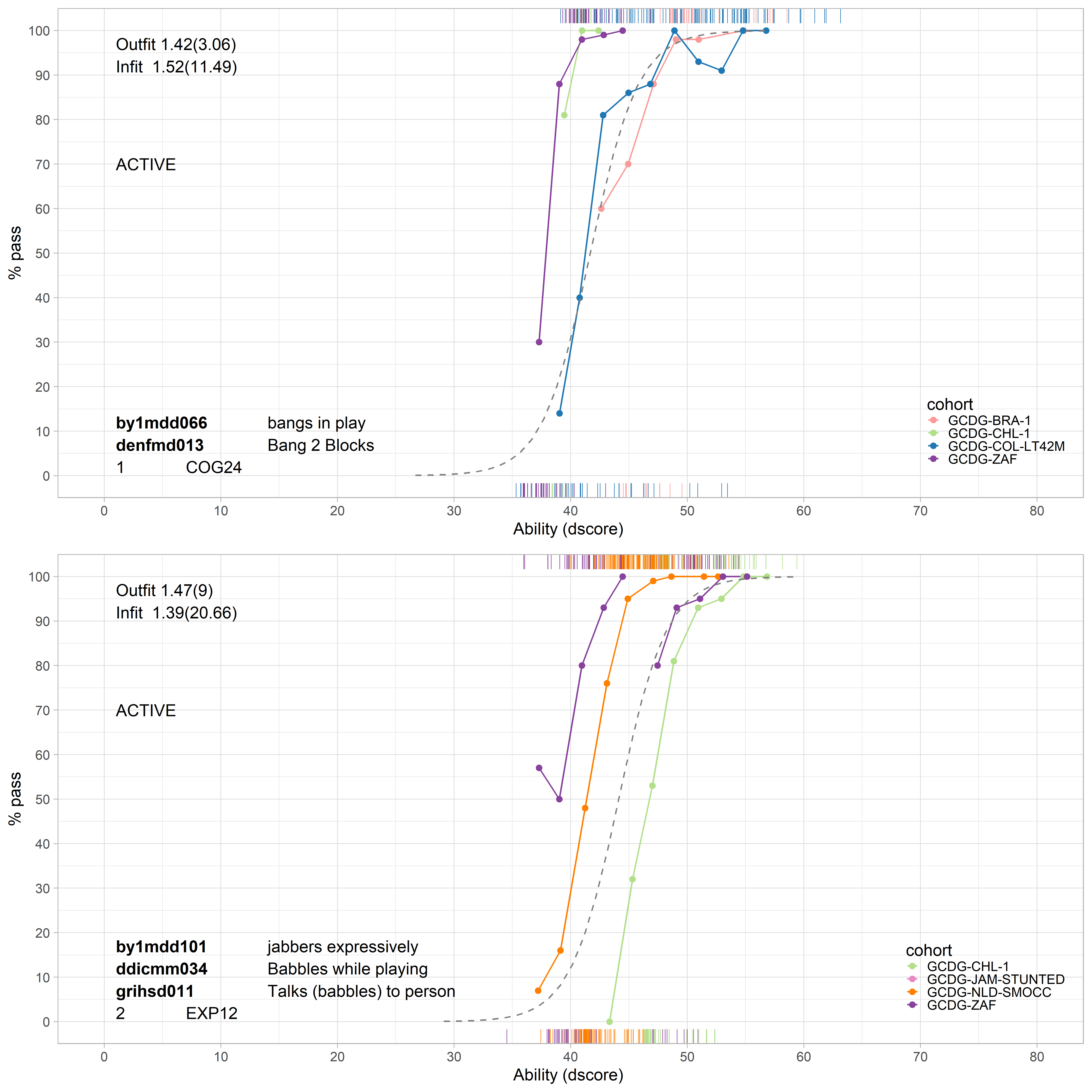
Figure 4.5: Two equate groups that present a poor equate fit.

Figure 4.5 shows examples for groups COG24 (Bangs in play / Bangs 2 blocks) and EXP12 (Babbles). In both cases there is substantial variation in location between the empirical curves. For COG24 we find that the fitted curve is closer to the den item, which suggests that the equate difficulty is mostly based on the den item. Items from equate group EXP12 have a different format in instruments by1, ddi, and gri. The empirical curves, with different colours for each instrument, are not close to each other, nor close to the fitted curve. Note that all infit and outfit statistics are fairly high, indicating poor fit. Both equates are candidates for deactivation in a next modelling step.