Scoring GSED

D-score and DAZ

Suppose you have administered GSED SF, GSED LF (World Health Organization (WHO) 2023; McCray et al. 2023) or GSED HF to one or more children. The next step is calculating each child’s developmental score (D-score) and age-adjusted equivalent (DAZ). This step is known as scoring. The present section provides recipes for calculating the D-score and DAZ. We may pick one of the following two methods:

Online calculator. The online app D-score calculator is a convenient option for users not familiar with R. The app contains online documentation and instructions and will not be further discussed here.
R package dscore. The R package dscore at https://CRAN.R-project.org/package=dscore is a flexible option with all the tools needed to calculate the D-score. It is an excellent choice for users familiar with R and users who like to incorporate D-score calculations into a workflow.

Preliminaries

We use the R language. If you are new to R consult the R for Data Science book by Hadley Wickham and Garrett Grolemund;
You need to install the R package dscore on your local machine;
The child data need to be stored as a data.frame, a standard R tabular structure;
You need to run the dscore() function to calculate the D-score and DAZ. The function returns a table with six columns with the estimates with the same number of rows as your data.

Install the `dscore` package

The dscore package contains tools to

Map your item names to the GSED convention
Calculate D-scores from item level responses
Transform the D-scores into DAZ, age-standardised Z-scores

The required input consists of item level responses on milestones collected using instruments for measuring child development, including the GSED LF, GSED SF and GSED HF.

There are two versions of the dscore package. For daily use, we recommend the curated and published version on CRAN. In R, install the dscore package as

install.packages("dscore")

In some cases, you might need a more recent version that includes extensions and bug fixes not yet available on CRAN. You can install the development version from GitHub by:

install.packages("remotes")
remotes::install_github("d-score/dscore")

The development version requires a local C++ compiler for building the package from source.

GSED 9-position item names

The dscore() function accepts item names that follow the GSED 9-position schema. A name with a length of nine characters identifies every milestone. The following table shows the construction of names.

Position	Description	Example
1-3	instrument	`by3`
4-5	developmental domain	`cg`
6	administration mode	`d`
7-9	item number	`018`

Thus, item by3cgd018 refers to the 18th item in the cognitive scale of the Bayley-III. The label of the item can be obtained by

library(dscore)
get_labels("by3cgd018")

##           by3cgd018 
## "Inspects own hand"

The dscore package maintains a list of items names.

Response data format

Rows: One measurement, i.e., one test administration for a child at a given age, occupies a row in the data set. Thus, if a child is measured three times at different ages, there will be three rows for that child in the dataset.

Columns: There should be at least two columns in the data set:

One column with the age of the child. The age column may have any name, and may be measured in decimal age, months, or days since birth. Do not truncate age. Make the value as a continuous as possible, for example by calculating age in days by the difference between measurement date and birth date.
One column for each item, appropriately named by the 9-position GSED item name. Normally, the items come from the same instrument, but they may also come from multiple instruments. The data from any recognised item name will contribute to the D-score. Do not duplicate names in the data. A PASS is coded as 1, a FAIL as 0. If there is no answer or if the item was not administered use the missing value code NA. Items that are never administered may be coded as all NA or deleted.

The dataset may contain additional columns, e.g., the child number or health information. These are ignored by the D-score calculation.

The most important steps is preparing the data for the D-score calculations are:

rename your original variable names into the 9-position GSED item names;
recode all item response as 0, 1 or NA

GSED Instruments

The table below lists the five available GSED instruments:

Instrument	Year	Code	Domains	Mode	Range	Status
GSED SF	2023	`gs1`	`cg\|lg\|li\|mo\|se`	`c`	`001-139`	Active
GSED LF	2023	`gl1`	`gm\|lg\|fm`	`d`	`001-049\|052\|054`	Active
GSED HF	2023	`gh1`	`cg\|lg\|li\|mo\|se`	`c`	`001-048`	Active
GSED SF	2020	`gpa`	any	`c`	`001-139`	Retired
GSED LF	2020	`gto`	`gm\|lg\|fm`	`d`	`001-049\|052\|054`	Retired

Instruments

`GSED SF`

The GSED Short Form (GSED SF) is a caregiver-reported instrument containing 139 items. It has instrument code gs1.

Check

Obtain the full list of item name for as

instrument <- "gs1"
items <- get_itemnames(instrument = instrument, order = "indm")
length(items)

## [1] 139

head(items)

## [1] "gs1sec001" "gs1moc002" "gs1sec003" "gs1lgc004" "gs1moc005" "gs1cgc006"

The order argument is needed to sort items according to sequence number 1 to 139. Check that you have the correct version by comparing the labels of the first few items as:

labels <- get_labels(items)
head(cbind(items, substr(labels, 1, 50)))

##           items                                                           
## gs1sec001 "gs1sec001" "SF001 Does your child smile?"                      
## gs1moc002 "gs1moc002" "SF002 When lying on his/her back, does your child "
## gs1sec003 "gs1sec003" "SF003 Does your child look at your face when you s"
## gs1lgc004 "gs1lgc004" "SF004 Does your child cry when he/she is hungry, w"
## gs1moc005 "gs1moc005" "SF005 Does your child grasp your finger if you tou"
## gs1cgc006 "gs1cgc006" "SF006 Does your child look at and focus on objects"

Renaming example

Suppose that you stored your data with items names sf001 to sf139. For example,

sf <- dscore::sample_sf
head(sf[, c(1:2, 101:105)])

##   subjid agedays sf099 sf100 sf101 sf102 sf103
## 1      1     811     1     1     1     1     1
## 2      2     898     1     1     1     1     1
## 3      3     203    NA    NA    NA    NA    NA
## 4      4     966    NA    NA    NA     1    NA
## 5      8     770     1     1     1     0     1
## 6      9     306    NA    NA    NA    NA    NA

Make sure that the items are in the correct order. Rename the columns with gsed 9-position item names.

colnames(sf)[3:141] <- items
head(sf[, c(1:2, 101:105)])

##   subjid agedays gs1lgc099 gs1lgc100 gs1moc101 gs1sec102 gs1lic103
## 1      1     811         1         1         1         1         1
## 2      2     898         1         1         1         1         1
## 3      3     203        NA        NA        NA        NA        NA
## 4      4     966        NA        NA        NA         1        NA
## 5      8     770         1         1         1         0         1
## 6      9     306        NA        NA        NA        NA        NA

The data in sf are now ready for the dscore() function.

Calculate D-score

Once the data are in proper shape, calculation of the D-score is straightforward. The sf dataset has properly named columns that identify each item.

results <- dscore(sf, xname = "agedays", xunit = "days")
head(results)

##        a  n      p     d      sem    daz
## 1 2.2204 29 0.7586 67.67 1.658818 -0.043
## 2 2.4586 39 0.6923 69.05 1.411819 -0.352
## 3 0.5558 48 0.6667 38.97 1.649425  1.058
## 4 2.6448 36 0.7500 74.47 1.471799  0.624
## 5 2.1081 50 0.5000 66.45 1.244876 -0.033
## 6 0.8378 48 0.7083 42.18 1.699459 -0.839

The table below provides the interpretation of the output:

Name	Interpretation
`a`	Decimal age in years
`n`	Number of items used to calculate the D-score
`p`	Proportion of passed milestones
`d`	D-score (posterior mean)
`sem`	Standard error of measurement (posterior standard deviation)
`daz`	D-score corrected for age

The number of rows of result is equal to the number of rows of sf. We save the result for later processing.

sf2 <- data.frame(sf, results)

It is possible to calculate D-score for item subsets by setting the items argument. We do not advertise this option for practical application, but suppose we are interested in the D-score based on items from gs1 and gl1 for domains mo or gm (motor) only. The “motor” D-score can be calculated as follows:

items_motor <- get_itemnames(
  instrument = c("gs1", "gl1"),
  domain = c("mo", "gm")
)
results <- dscore(sf, items = items_motor, xname = "agedays", xunit = "days")
head(results)

##        a  n      p     d      sem    daz
## 1 2.2204  6 0.8333 67.40 3.391252 -0.116
## 2 2.4586  8 0.7500 69.16 3.049288 -0.324
## 3 0.5558 30 0.7333 39.89 1.946849  1.347
## 4 2.6448  5 0.8000 75.78 3.154717  0.981
## 5 2.1081 10 0.7000 69.52 2.808620  0.814
## 6 0.8378 31 0.7419 42.35 1.983714 -0.790

`GSED LF`

The GSED Long Form (GSED LF) instrument is a directly-observed instrument containing 155 items with instrument code gl1.

Check

Obtain the full list of item name for as

instrument <- "gl1"
items <- get_itemnames(instrument = instrument)
length(items)

## [1] 155

head(items)

## [1] "gl1fmd001" "gl1fmd002" "gl1fmd003" "gl1fmd004" "gl1fmd005" "gl1fmd006"

Reorder item names so that they corresponds to streams A, B and C, respectively.

items <- items[c(55:155, 1:54)]
head(items)

## [1] "gl1gmd001" "gl1gmd002" "gl1gmd003" "gl1gmd004" "gl1gmd005" "gl1gmd006"

Check that you have the correct version by comparing the labels of the first few items as:

labels <- get_labels(items)
head(cbind(items, substr(labels, 1, 50)))

##           items                                                           
## gl1gmd001 "gl1gmd001" "A1  Moves body in reaction to caregiver"           
## gl1gmd002 "gl1gmd002" "A2  Moves body, kicking legs and moving arms equal"
## gl1gmd003 "gl1gmd003" "A3  Pulls to sit - no head lag"                    
## gl1gmd004 "gl1gmd004" "A4  Lifts head in prone 45 degrees (2X)"           
## gl1gmd005 "gl1gmd005" "A5  Lifts head, shoulders, chest when prone (2X)"  
## gl1gmd006 "gl1gmd006" "A6  Puts hands together in front of face"

Renaming example

Suppose that you stored your data with items names lf001 to lf155. For example,

lf <- dscore::sample_lf
head(lf[, c(1:2, 60:64)])

##   subjid agedays lf058 lf059 lf060 lf061 lf062
## 1      1     811    NA    NA    NA    NA    NA
## 2      2     898    NA    NA    NA    NA    NA
## 3      3     203     0     0     0    NA    NA
## 4      4     966    NA    NA    NA    NA    NA
## 5      8     770     0     0     0     0     0
## 6      9     306     1     1     0     1     0

Make sure that the items are in the correct order. Rename the columns with gsed 9-position item names.

colnames(lf)[3:157] <- items
head(lf[, c(1:2, 60:64)])

##   subjid agedays gl1lgd009 gl1lgd010 gl1lgd011 gl1lgd012 gl1lgd013
## 1      1     811        NA        NA        NA        NA        NA
## 2      2     898        NA        NA        NA        NA        NA
## 3      3     203         0         0         0        NA        NA
## 4      4     966        NA        NA        NA        NA        NA
## 5      8     770         0         0         0         0         0
## 6      9     306         1         1         0         1         0

The data in lf are now ready for the dscore() function.

Calculate D-score

Once the data are in proper shape, calculation of the D-score is straightforward. The lf dataset has properly named columns that identify each item.

results <- dscore(lf, xname = "agedays", xunit = "days")
head(results)

##        a  n      p     d      sem    daz
## 1 2.2204 42 0.5476 66.91 1.328849 -0.246
## 2 2.4586 49 0.6122 70.69 1.239337  0.082
## 3 0.5558 31 0.5484 34.27 1.661074 -0.397
## 4 2.6448 52 0.5000 70.11 1.165718 -0.529
## 5 2.1081 53 0.1509 40.67 1.820166 -4.554
## 6 0.8378 31 0.5806 44.85 1.554783 -0.038

The table below provides the interpretation of the output:

Name	Interpretation
`a`	Decimal age in years
`n`	Number of items used to calculate the D-score
`p`	Proportion of passed milestones
`d`	D-score (posterior mean)
`sem`	Standard error of measurement (posterior standard deviation)
`daz`	D-score corrected for age

The number of rows of result is equal to the number of rows of lf. We save the result for later processing.

lf2 <- data.frame(lf, results)

items_motor <- get_itemnames(
  instrument = c("gs1", "gl1"),
  domain = c("mo", "gm")
)
results <- dscore(lf, items = items_motor, xname = "agedays", xunit = "days")
head(results)

##        a  n      p     d      sem    daz
## 1 2.2204 12 0.5833 64.88 2.844278 -0.772
## 2 2.4586 17 0.6471 70.62 2.244729  0.063
## 3 0.5558 19 0.6842 36.27 2.010557  0.213
## 4 2.6448 12 0.4167 65.46 2.707788 -1.626
## 5 2.1081 12 0.5000 60.25 2.784830 -1.589
## 6 0.8378 14 0.7143 45.20 2.350039  0.070

`GSED HF`

The GSED Houshold Form (GSED HF) instrument contains a subset of 48 items from the GSED SF designed to be used for population surveys. It has instrument code gh1.

Check

Obtain the full list of item name for as

instrument <- "gh1"
items <- get_itemnames(instrument = instrument, order = "indm")
length(items)

## [1] 48

head(items)

## [1] "gh1lgc001" "gh1sec002" "gh1lgc003" "gh1sec004" "gh1moc005" "gh1lgc006"

The order argument is needed to sort items according to sequence number 1 to 48. Check that you have the correct version by comparing the labels of the first few items as:

labels <- get_labels(items)
head(cbind(items, substr(labels, 1, 50)))

##           items                                                           
## gh1lgc001 "gh1lgc001" "HF001 When you talk to your child, does he/she smi"
## gh1sec002 "gh1sec002" "HF002 When you are about to pick up your child, do"
## gh1lgc003 "gh1lgc003" "HF003 Does your child turn his/her head towards yo"
## gh1sec004 "gh1sec004" "HF004 Does your child sometimes suck his/her thumb"
## gh1moc005 "gh1moc005" "HF005 While your child is on his/her back, can he/"
## gh1lgc006 "gh1lgc006" "HF006 Does your child make noise or gesture to get"

Renaming example

Suppose that you stored your data with items names hf001 to hf048. For example,

hf <- dscore::sample_hf
head(hf[, c(1:2, 30:35)])

##   subjid agedays hf028 hf029 hf030 hf031 hf032 hf033
## 1      1     811    NA    NA    NA    NA    NA    NA
## 2      2     898    NA    NA    NA    NA    NA    NA
## 3      3     203     0    NA     0    NA     0     0
## 4      4     966    NA    NA    NA    NA    NA    NA
## 5      8     770    NA    NA    NA    NA    NA    NA
## 6      9     306     0     0     0    NA     0     0

Make sure that the items are in the correct order. Rename the columns with gsed 9-position item names.

colnames(hf)[3:50] <- items
head(hf[, c(1:2, 30:35)])

##   subjid agedays gh1moc028 gh1lgc029 gh1moc030 gh1sec031 gh1moc032 gh1moc033
## 1      1     811        NA        NA        NA        NA        NA        NA
## 2      2     898        NA        NA        NA        NA        NA        NA
## 3      3     203         0        NA         0        NA         0         0
## 4      4     966        NA        NA        NA        NA        NA        NA
## 5      8     770        NA        NA        NA        NA        NA        NA
## 6      9     306         0         0         0        NA         0         0

The data in hf are now ready for the dscore() function.

Calculate D-score

Once the data are in proper shape, calculation of the D-score is straightforward. The hf dataset has properly named columns that identify each item.

results <- dscore(hf, xname = "agedays", xunit = "days", verbose = TRUE)

## key:         gsed2510 
## population:  preliminary_standards 
## transform:   55.72413 3.603965 
## qp range:    -10 125 
## algorithm:   current 
## key:         gsed2510 
## population:  preliminary_standards

head(results)

##        a  n      p     d      sem    daz
## 1 2.2204  8 0.7500 66.80 2.867389 -0.275
## 2 2.4586  8 1.0000 73.81 3.837050  0.934
## 3 0.5558 27 0.5926 37.46 2.139379  0.583
## 4 2.6448  3 1.0000 74.35 4.116044  0.591
## 5 2.1081  7 1.0000 71.00 3.706083  1.227
## 6 0.8378 28 0.6429 41.51 2.081210 -1.032

The table below provides the interpretation of the output:

Name	Interpretation
`a`	Decimal age in years
`n`	Number of items used to calculate the D-score
`p`	Proportion of passed milestones
`d`	D-score (posterior mean)
`sem`	Standard error of measurement (posterior standard deviation)
`daz`	D-score corrected for age

The number of rows of results is equal to the number of rows of hf. We save the result for later processing.

hf2 <- data.frame(hf, results)

It is possible to calculate D-score for item subsets by setting the items argument. We do not advertise this option for practical application, but suppose we are interested in the D-score based on items from gs1, gl1 and gh1 for domains mo or gm (motor) only. The “motor” D-score can be calculated as follows:

items_motor <- get_itemnames(
  instrument = c("gs1", "gl1", "gh1"),
  domain = c("mo", "gm")
)
results <- dscore(
  hf,
  items = items_motor,
  xname = "agedays",
  xunit = "days",
)
head(results)

##        a  n      p     d      sem    daz
## 1 2.2204  1 1.0000 69.67 4.442820  0.502
## 2 2.4586  1 1.0000 71.51 4.543754  0.303
## 3 0.5558 18 0.5000 36.88 2.414803  0.402
## 4 2.6448  1 1.0000 72.83 4.615730  0.181
## 5 2.1081  1 1.0000 68.73 4.395200  0.594
## 6 0.8378 18 0.5556 40.84 2.399928 -1.221

Other GSED instruments

The gpa (SF) and gto (LF) instrument codes are included only for backward compatibility. These instruments have a different item order. They were replaced in 2023 by the GSED SF (gs1) and GSED LF (gl1). The scoring procedure is identical to the one described above for the new instruments.

References for DAZ calculation

`preliminary_standards` references

By default, DAZ values are calculated using the preliminary standards. These standards were derived from a healthy subsample of approximately 12,000 administrations of the GSED SF and GSED LF collected in Bangladesh, Pakistan, and Tanzania (the GSED Phase 1 countries), using the key “gsed2406”. You can extract these reference values with:

library(dplyr, warn.conflicts = FALSE, quietly = TRUE)
ref <- builtin_references |>
  filter(population == "preliminary_standards") |>
  select(population, age, mu, sigma, nu, tau, SDM2, SD0, SDP2) |>
  mutate(m = age * 12)

head(ref, 3)

##              population    age    mu  sigma    nu    tau     SDM2      SD0
## 1 preliminary_standards 0.0000 11.46 0.2075 1.420 34.189 5.941355 11.46264
## 2 preliminary_standards 0.0383 13.18 0.2075 1.420 34.189 6.833076 13.18304
## 3 preliminary_standards 0.0575 14.04 0.2001 1.426 34.121 7.529790 14.04231
##       SDP2      m
## 1 16.03876 0.0000
## 2 18.44597 0.4596
## 3 19.45665 0.6900

The columns mu, sigma, nu and tau are the age-varying parameters of a Box-Cox $t$ (BCT) distribution.

The references are currently also available for the updated key "gsed2510", which is the recommended key for GSED instruments.
A future release of the package will replace the current preliminary_standards for "gsed2510" with a newly calculated version based on data from all seven GSED countries.

You do not need to manually specify the references when calculating DAZ with the dscore() function. The function automatically uses the preliminary_standards references. For example, you can calculate the D-score and DAZ as follows:

vars <- c("id", "agedays", get_itemnames(instrument = "gs1", order = "indm"))
data <- triple[, colnames(triple) %in% vars]
ds1 <- dscore(data, xname = "agedays", xunit = "days")
head(ds1)

##        a  n      p     d      sem    daz
## 1 1.9493 65 0.6769 68.95 1.210561  1.186
## 2 2.5325 34 0.7059 73.23 1.458141  0.572
## 3 2.3874 36 0.5833 65.89 1.404537 -0.966
## 4 0.8980  8 0.5000 38.64 2.527097 -2.228
## 5 2.1903 31 0.2258 57.84 1.605532 -2.289
## 6 0.8980 80 0.7625 54.78 1.325298  2.517

Add the argument dscore(..., verbose = TRUE) to see which references are used.

Here are the growth charts for D-score and DAZ, based on the preliminary_standards references.

library(ggplot2)
library(patchwork)

r <- builtin_references |>
  filter(population == "preliminary_standards" & age <= 3.5) |>
  mutate(m = age * 12)

ds1$m <- ds1$a * 12
g1 <- ggplot(ds1, aes(x = m, y = d)) +
  theme_light() +
  annotate(
    "polygon",
    x = c(r$age, rev(r$age)),
    y = c(r$SDM2, rev(r$SDP2)),
    alpha = 0.06,
    fill = "#C5EDDE"
  ) +
  annotate("line", x = r$m, y = r$SDM2, lwd = 0.5, color = "grey80") +
  annotate("line", x = r$m, y = r$SDP2, lwd = 0.5, color = "grey80") +
  annotate("line", x = r$m, y = r$SD0, lwd = 1, color = "grey80") +
  scale_x_continuous(
    "Age (in months)",
    limits = c(0, 42),
    breaks = seq(0, 42, 12)
  ) +
  scale_y_continuous(
    expression(paste("D-score", sep = "")),
    breaks = seq(0, 80, 20),
    limits = c(0, 90)
  ) +
  geom_point(size = 2) +
  theme(legend.position = "none")
g2 <- ggplot(ds1, aes(x = m, y = daz)) +
  theme_light() +
  geom_hline(yintercept = 2, linewidth = 0.5, color = "grey80") +
  geom_hline(yintercept = -2, linewidth = 0.5, color = "grey80") +
  geom_hline(yintercept = 0, linewidth = 1.0, color = "grey80") +
  scale_x_continuous(
    "Age (in months)",
    limits = c(0, 42),
    breaks = seq(0, 42, 12)
  ) +
  scale_y_continuous(
    "DAZ",
    breaks = seq(-4, 4, 2),
    limits = c(-4, 4)
  ) +
  geom_point(size = 2) +
  theme(legend.position = "none")
g1 + g2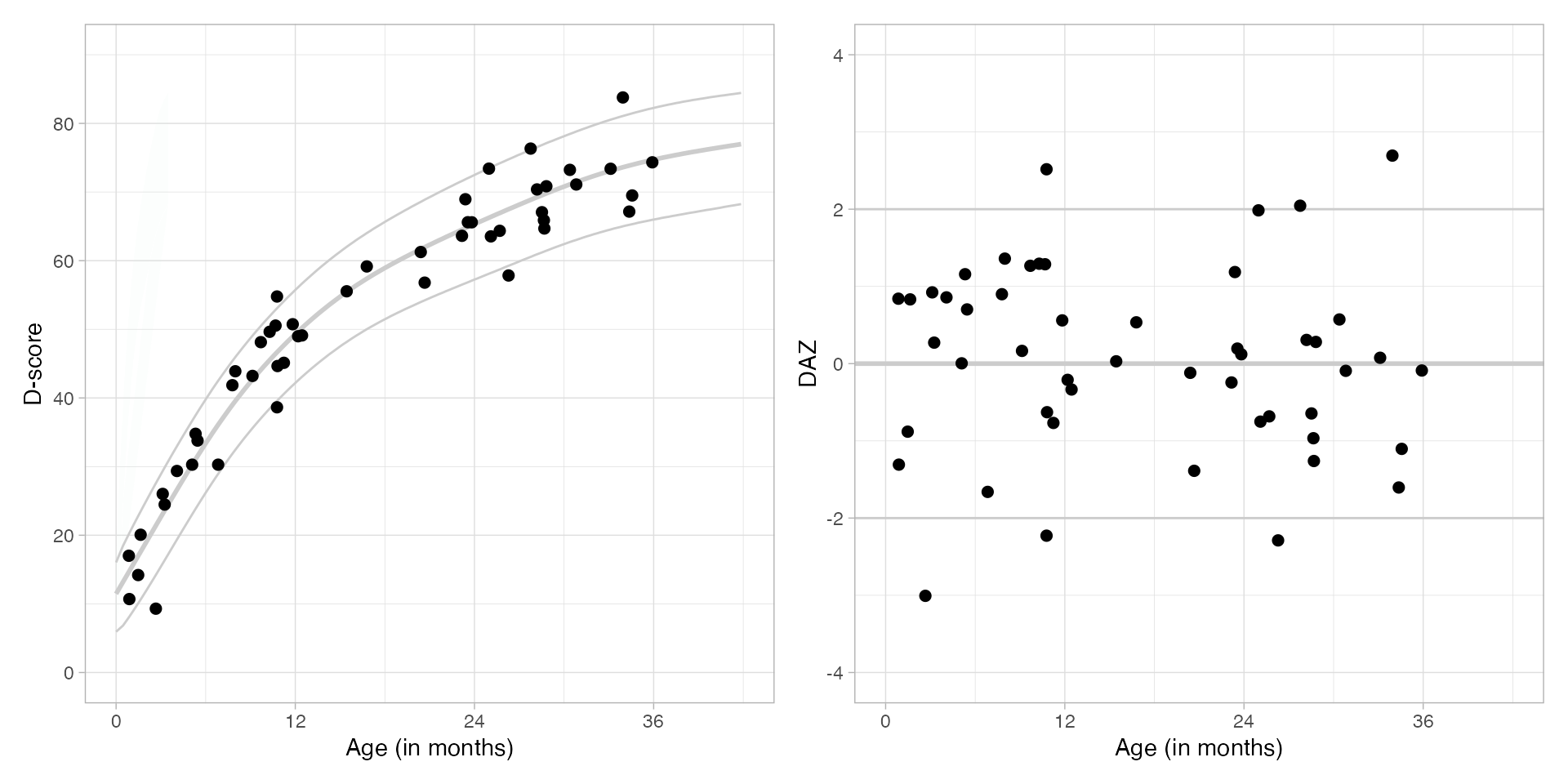

`who_descriptive` references

The who_descriptive references are based on data from all children across all seven GSED countries. These references reflect the observed data and should not be interpreted as standards. They are intended for descriptive analyses of developmental status or for methodological studies.

The who_descriptive references replace the earlier "phase1" references, which were derived from GSED Phase I data (three countries).

You can access these references by specifying population = "who_descriptive" in the dscore() function. To extract the references, use:

ref <- builtin_references |>
  filter(population == "who_descriptive") |>
  select(population, age, mu, sigma, nu, tau, SDM2, SD0, SDP2)
head(ref)

##        population    age    mu  sigma     nu    tau     SDM2      SD0     SDP2
## 1 who_descriptive 0.0000 11.61 0.2620 0.9079 21.068 5.354991 11.61077 18.22228
## 2 who_descriptive 0.0192 12.40 0.2519 0.9310 21.106 5.919198 12.40068 19.14714
## 3 who_descriptive 0.0383 13.20 0.2422 0.9541 21.144 6.511667 13.20059 20.06532
## 4 who_descriptive 0.0575 14.00 0.2329 0.9772 21.182 7.126490 14.00051 20.96359
## 5 who_descriptive 0.0767 14.80 0.2239 1.0008 21.220 7.764326 14.80044 21.84040
## 6 who_descriptive 0.0958 15.60 0.2153 1.0253 21.257 8.420108 15.60038 22.70040

The columns mu, sigma, nu and tau are the age-varying parameters of a Box-Cox $t$ (BCT) distribution.

ds2 <- dscore(
  data,
  xname = "agedays",
  xunit = "days",
  population = "who_descriptive"
)
head(ds2)

##        a  n      p     d      sem    daz
## 1 1.9493 65 0.6769 68.95 1.210561  1.030
## 2 2.5325 34 0.7059 73.23 1.458141  0.559
## 3 2.3874 36 0.5833 65.89 1.404537 -1.027
## 4 0.8980  8 0.5000 38.64 2.527097 -2.018
## 5 2.1903 31 0.2258 57.84 1.605532 -2.435
## 6 0.8980 80 0.7625 54.78 1.325298  2.578

Here are the growth charts for D-score and DAZ, based on the who_descriptive references.

library(ggplot2)
library(patchwork)

r <- builtin_references |>
  filter(population == "who_descriptive" & age <= 3.5) |>
  mutate(m = age * 12)

ds2$m <- ds2$a * 12
g1 <- ggplot(ds2, aes(x = m, y = d)) +
  theme_light() +
  annotate(
    "polygon",
    x = c(r$age, rev(r$age)),
    y = c(r$SDM2, rev(r$SDP2)),
    alpha = 0.06,
    fill = "#C5EDDE"
  ) +
  annotate("line", x = r$m, y = r$SDM2, lwd = 0.5, color = "grey80") +
  annotate("line", x = r$m, y = r$SDP2, lwd = 0.5, color = "grey80") +
  annotate("line", x = r$m, y = r$SD0, lwd = 1, color = "grey80") +
  scale_x_continuous(
    "Age (in months)",
    limits = c(0, 42),
    breaks = seq(0, 42, 12)
  ) +
  scale_y_continuous(
    expression(paste("D-score", sep = "")),
    breaks = seq(0, 80, 20),
    limits = c(0, 90)
  ) +
  geom_point(size = 2) +
  theme(legend.position = "none")
g2 <- ggplot(ds2, aes(x = m, y = daz)) +
  theme_light() +
  geom_hline(yintercept = 2, linewidth = 0.5, color = "grey80") +
  geom_hline(yintercept = -2, linewidth = 0.5, color = "grey80") +
  geom_hline(yintercept = 0, linewidth = 1.0, color = "grey80") +
  scale_x_continuous(
    "Age (in months)",
    limits = c(0, 42),
    breaks = seq(0, 42, 12)
  ) +
  scale_y_continuous(
    "DAZ",
    breaks = seq(-4, 4, 2),
    limits = c(-4, 4)
  ) +
  geom_point(size = 2) +
  theme(legend.position = "none")
g1 + g2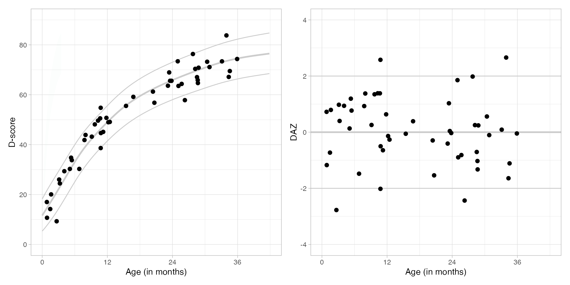

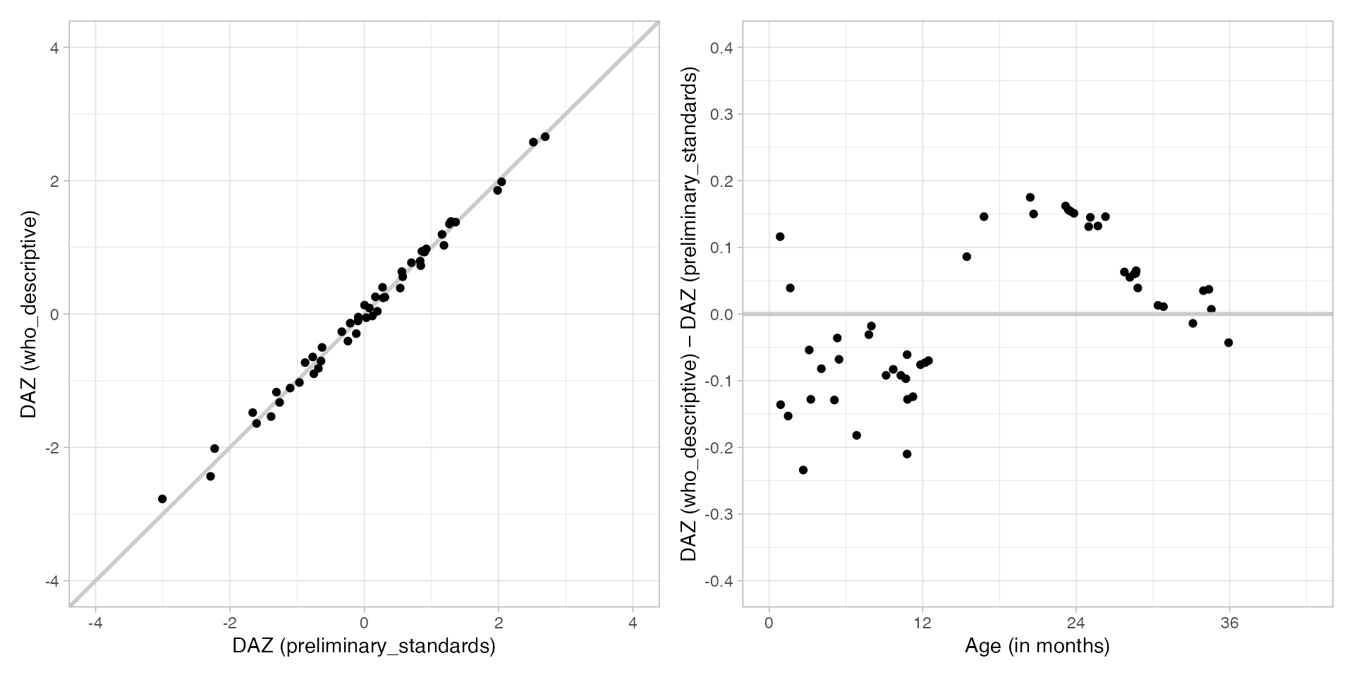
In general, descriptive references are expected to yield higher DAZ values than standards. This is because descriptive references are based on all children, including those with developmental delays, whereas standards are based on a healthy subsample.

At present, the who_descriptive references produce DAZ values similar to those from the preliminary_standards references, but with a noticeably different age pattern. The main reason is that who_descriptive is based on key gsed2510, while preliminary_standards still rely on the older key gsed2406. This age pattern is expected to disappear once the new standards based on key gsed2510 become available.

f1 <- ggplot(data = NULL, aes(x = ds1$daz, y = ds2$daz)) +
  theme_light() +
  geom_abline(intercept = 0, slope = 1, colour = "grey80", linewidth = 1) +
  geom_point(shape = 19) +
  scale_y_continuous(
    "DAZ (who_descriptive)",
    breaks = seq(-4, 4, 2),
    limits = c(-4, 4)
  ) +
  scale_x_continuous(
    "DAZ (preliminary_standards)",
    breaks = seq(-4, 4, 2),
    limits = c(-4, 4)
  )

f2 <- ggplot(data = NULL, aes(x = ds1$a * 12, y = ds1$daz - ds2$daz)) +
  theme_light() +
  geom_point(shape = 19) +
  geom_hline(yintercept = 0, colour = "grey80", linewidth = 1) +
  scale_x_continuous(
    "Age (in months)",
    limits = c(0, 42),
    breaks = seq(0, 42, 12)
  ) +
  scale_y_continuous(
    "DAZ (who_descriptive) – DAZ (preliminary_standards)",
    breaks = seq(-0.4, 0.4, 0.1),
    limits = c(-0.4, 0.4)
  )

f1 + f2

Literature references

McCray, G, D McCoy, P Kariger, M Janus, MM Black, SM Chang, F Tofail, et al. 2023. “The Creation of the Global Scales for Early Development (GSED) for Children Aged 0-3 Years: Combining Subject Matter Expert Judgements with Big Data.” BMJ Glob Health 8 (1).

World Health Organization (WHO). 2023. “Global Scales for Early Development (GSED) V1.0: Technical Report.” Geneva: World Health Organization. https://www.who.int/publications/i/item/WHO-MSD-GSED-package-v1.0-2023.1.

D-score and DAZ

Preliminaries

Install the dscore package

GSED 9-position item names

Response data format

GSED Instruments

Instruments

GSED SF

Check

Renaming example

Calculate D-score

GSED LF

Check

Renaming example

Calculate D-score

GSED HF

Check

Renaming example

Calculate D-score

Other GSED instruments

References for DAZ calculation

preliminary_standards references

who_descriptive references

Literature references

Install the `dscore` package

`GSED SF`

`GSED LF`

`GSED HF`

`preliminary_standards` references

`who_descriptive` references