Overview
The D-score is a one-number summary measure of early child development. The D-score has a fixed unit. In principle, we may use the D-score to answer questions on the individual, group and population level, but be aware that no instruments have yet been validated for individual application. For more background, see the introductory booklet D-score: Turning milestones into measurement.
This vignette shows how to estimate the D-score and the D-score age-adjusted Z-score (DAZ) from child data on developmental milestones. The vignette covers some typical actions needed when estimating the D-score and DAZ:
- Identify whether the
dscorepackage covers your measurement instrument; - Map your variable names to the GSED 9-position schema;
- Calculate D-score and DAZ;
- Summarise your results.
Is your measurement instrument covered?
The dscore package covers a subset of all possible
assessment instruments. Moreover, it may have a restricted age range for
a given instrument. Your first task is to evaluate whether the current
dscore package can convert your measurements into
D-scores.
A 2017 Worldbank report (Fernald et al. 2017) identified 147 instruments for assessing the development of children aged 0-8 years. Well-known examples include the Bayley Scales for Infant and Toddler Development and the Ages & Stages Questionnaires. The D-score is defined by and calculated from, subsets of milestones from such instruments.
Assessment instruments connect to the D-score through a measurement model, the Rasch model. We use the term key to refer to a particular set of parameters (difficulty estimates) of a fitted Rasch model. The key defines how 0/1 milestone scores are translated into a D-score, as thus can be seen as part of the scoring system.
The dscore package contains a generic algorithm that
takes:
- the 0/1 scores on a set of milestones for a given child;
- the age(s) of the child at which the test is administered;
- a specification of the key;
and then calculates the D-score and its Standard Error of Measurement (SEM) for the child at each age.
The dscore package currently supports the following keys
(in historic order):
| Key name | Description | Reference |
|---|---|---|
dutch |
A model developed for the Dutch development instrument | S. van Buuren (2014) |
gcdg |
A model covering 13 instruments using direct measurements | Weber et al. (2019) |
gsed1912 |
Covers 20 instruments using a mix of direct and caregiver-reported measurements | Stef van Buuren et al. (2025) (Study 1) |
gsed2212 |
Covers 23 instruments using a mix of direct and caregiver-reported measurements | Stef van Buuren et al. (2025) (Study 2) |
gsed2406 |
Covers 23 instruments using a mix of direct and caregiver-reported measurements. Same as gsed2212, but with a different base population. | Stef van Buuren et al. (2025) (Study 2) |
gsed2510 |
Currently covers 4 instruments - In development | In preparation (Study 3) |
Different keys lead to (slightly) different D-scores. We may only compare D-scores that are calculated under the same key. Our advice to set the key is:
- For new data, use the generic
key = "gsed". This choice will automatically fetch the latest GSED key, which iskey = "gsed2510"; - Key
gsed2406has a wider coverage, Use that if your instrument is not covered bygsed2510. - Use older keys
dutch,gcdgorgsed1912to regenerate old results. These are unlikely to be useful for new data; - Superseded keys are:
gsed2212,gsed2206,gsed2208,lf2206,sf2006,294_0and293_0. Use for research purposes only.
The table given below displays the number of items per instrument for various keys. If the entry is blank, the key does not cover the instrument.
| Code | Instrument | Items | dutch | gcdg | gsed1912 | gsed2406 | gsed2510 |
|---|---|---|---|---|---|---|---|
aqi |
Ages & Stages Questionnaires-3 | 230 | 29 | 17 | 17 | ||
bar |
Barrera Moncada | 22 | 15 | 13 | 13 | ||
bat |
Battelle Development Inventory and Screener-2 | 137 | |||||
by1 |
Bayley Scales for Infant and Toddler Development-1 | 156 | 85 | 76 | 76 | ||
by2 |
Bayley Scales for Infant and Toddler Development-2 | 121 | 16 | 16 | 16 | ||
by3 |
Bayley Scales for Infant and Toddler Development-3 | 320 | 105 | 67 | 172 | 242 | |
cro |
Caregiver Reported Early Development Instrument (CREDI) | 149 | 62 | 64 | |||
ddi |
Dutch Development Instrument (Van Wiechen Schema) | 77 | 76 | 65 | 64 | 64 | |
den |
Denver-2 | 111 | 67 | 50 | 50 | ||
dmc |
Developmental Milestones Checklist | 66 | 43 | 43 | |||
gri |
Griffiths Mental Development Scales | 312 | 104 | 93 | 18 | ||
gs1 |
GSED SF (2023) | 139 | 138 | 136 | |||
gl1 |
GSED LF (2023) | 155 | 155 | 145 | |||
gh1 |
GSED HF (2023) | 48 | 48 | 48 | |||
iyo |
Infant and Young Child Development (IYCD) | 90 | 55 | 57 | |||
kdi |
Kilifi Developmental Inventory | 69 | 48 | 48 | |||
mac |
MacArthur Communicative Development Inventory | 6 | 3 | 3 | 3 | ||
mds |
WHO Motor Development Milestones | 6 | 1 | 1 | |||
mdt |
Malawi Developmental Assessment Tool (MDAT) | 136 | 126 | 126 | |||
peg |
Pegboard | 2 | 1 | 1 | 1 | ||
pri |
Project on Child Development Indicators (PRIDI) | 63 | |||||
sbi |
Stanford Binet Intelligence Scales-4/5 | 33 | 6 | 5 | 5 | ||
sgr |
Griffiths for South Africa | 58 | 19 | 19 | 19 | ||
tep |
Test de Desarrollo Psicomotor (TEPSI) | 61 | 33 | 31 | 31 | ||
vin |
Vineland Social Maturity Scale | 50 | 17 | 17 | 17 | ||
| Extensions | |||||||
ecd |
Early Child Development Indicators (ECDI) | 20 | 18 | ||||
mul |
Mullen Scales of Early Learning | 232 | 138 |
You can’t compute a D-score if your instrument isn’t supported. If it does measure child development, we can often extend the key to include it. This requires a one-time effort—mapping your items to the milestone schema and estimating difficulty parameters. Once added, the key is reusable, and you’ll be able to compute valid D-scores for that instrument. The table shows two such extensions: one for Mullen and one for ECDI.
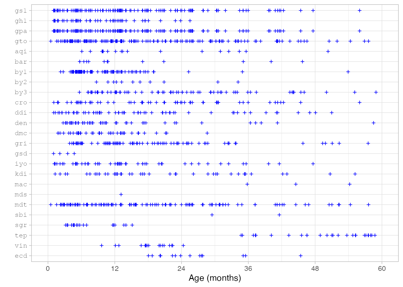
The designs of the original cohorts determine the age coverage for
each instrument. The figure above indicates the age range currently
supported by the "gsed2510" key.
GSED 9-position item names
The dscore() function accepts item names that follow the
GSED 9-position schema. A name with a length of nine characters
identifies every milestone. The following table shows the construction
of names.
| Position | Description | Example |
|---|---|---|
| 1-3 | instrument | by3 |
| 4-5 | developmental domain | cg |
| 6 | administration mode | d |
| 7-9 | item number | 018 |
Thus, item by3cgd018 refers to the 18th item in the
cognitive scale of the Bayley-III. The label of the item can be obtained
by
library(dscore)
get_labels("by3cgd018")
## by3cgd018
## "Inspects own hand"You may decompose item names into components as follows:
decompose_itemnames(c("by3cgd018", "denfmd014"))## instrument domain mode number
## 1 by3 cg d 018
## 2 den fm d 014This function returns a data.frame with four character
vectors for further processing.
The dscore package recognises 3836 item names. The
expression get_itemnames() returns a (long) vector of all
known item names. Let us study the table of instruments by domain:
items <- get_itemnames()
din <- decompose_itemnames(items) |>
  dplyr::filter(!instrument %in% c("gsd", "gpa", "gto", "rap"))
knitr::kable(with(din, table(instrument, domain)), format = "html") |>
kableExtra::column_spec(1, monospace = TRUE)| ad | cg | cl | cm | co | eh | ex | fa | fm | fr | gm | hd | hs | lg | li | md | mo | NA | pd | px | re | se | sl | vs | wm | xx | |
|---|---|---|---|---|---|---|---|---|---|---|---|---|---|---|---|---|---|---|---|---|---|---|---|---|---|---|
| aqi | 0 | 0 | 0 | 63 | 0 | 0 | 0 | 0 | 61 | 0 | 62 | 0 | 0 | 0 | 0 | 0 | 0 | 1 | 0 | 68 | 0 | 0 | 67 | 0 | 0 | 0 |
| bar | 0 | 0 | 0 | 0 | 0 | 0 | 0 | 0 | 0 | 0 | 0 | 0 | 0 | 0 | 0 | 0 | 0 | 0 | 0 | 0 | 0 | 0 | 0 | 0 | 0 | 66 |
| bat | 26 | 26 | 0 | 27 | 0 | 0 | 0 | 0 | 0 | 0 | 0 | 0 | 0 | 0 | 0 | 0 | 30 | 0 | 0 | 0 | 0 | 0 | 28 | 0 | 0 | 0 |
| by1 | 0 | 0 | 0 | 0 | 0 | 0 | 0 | 0 | 0 | 0 | 0 | 0 | 0 | 0 | 0 | 134 | 0 | 0 | 66 | 0 | 0 | 0 | 0 | 0 | 0 | 0 |
| by2 | 0 | 0 | 0 | 0 | 0 | 0 | 0 | 0 | 0 | 0 | 0 | 0 | 0 | 0 | 0 | 165 | 0 | 0 | 109 | 0 | 0 | 0 | 0 | 0 | 0 | 0 |
| by3 | 0 | 91 | 0 | 0 | 0 | 0 | 48 | 0 | 66 | 0 | 72 | 0 | 0 | 0 | 0 | 0 | 0 | 0 | 0 | 0 | 49 | 0 | 0 | 0 | 0 | 0 |
| cro | 0 | 0 | 51 | 0 | 0 | 0 | 0 | 0 | 0 | 0 | 0 | 0 | 0 | 0 | 0 | 0 | 39 | 0 | 0 | 0 | 0 | 59 | 0 | 0 | 0 | 0 |
| ddi | 0 | 0 | 0 | 27 | 0 | 0 | 0 | 0 | 27 | 0 | 27 | 0 | 0 | 0 | 0 | 0 | 0 | 0 | 0 | 0 | 0 | 0 | 0 | 0 | 0 | 0 |
| den | 0 | 0 | 0 | 0 | 0 | 0 | 0 | 0 | 29 | 0 | 32 | 0 | 0 | 39 | 0 | 0 | 0 | 0 | 0 | 0 | 0 | 0 | 25 | 0 | 0 | 0 |
| dmc | 0 | 0 | 0 | 0 | 0 | 0 | 0 | 0 | 11 | 0 | 17 | 0 | 0 | 11 | 0 | 0 | 0 | 0 | 0 | 0 | 0 | 0 | 27 | 0 | 0 | 0 |
| ecd | 0 | 0 | 0 | 0 | 0 | 0 | 0 | 0 | 0 | 0 | 0 | 0 | 0 | 0 | 0 | 0 | 0 | 0 | 0 | 0 | 0 | 0 | 0 | 0 | 0 | 20 |
| gh1 | 0 | 0 | 9 | 1 | 0 | 0 | 0 | 0 | 0 | 0 | 3 | 0 | 0 | 6 | 0 | 0 | 21 | 0 | 0 | 0 | 0 | 7 | 0 | 0 | 0 | 1 |
| gl1 | 0 | 0 | 0 | 0 | 0 | 0 | 0 | 0 | 54 | 0 | 49 | 0 | 0 | 52 | 0 | 0 | 0 | 0 | 0 | 0 | 0 | 0 | 0 | 0 | 0 | 0 |
| gri | 0 | 86 | 0 | 0 | 0 | 86 | 0 | 0 | 0 | 0 | 86 | 0 | 86 | 0 | 0 | 0 | 0 | 0 | 0 | 0 | 38 | 0 | 0 | 0 | 0 | 0 |
| gs1 | 0 | 11 | 0 | 0 | 0 | 0 | 0 | 0 | 0 | 0 | 0 | 0 | 0 | 39 | 12 | 0 | 56 | 0 | 0 | 0 | 0 | 21 | 0 | 0 | 0 | 0 |
| hyp | 0 | 0 | 0 | 0 | 0 | 0 | 0 | 0 | 0 | 0 | 5 | 0 | 0 | 0 | 0 | 0 | 0 | 0 | 0 | 0 | 0 | 0 | 0 | 0 | 0 | 0 |
| iyo | 0 | 0 | 0 | 0 | 0 | 0 | 0 | 0 | 0 | 0 | 0 | 0 | 0 | 30 | 0 | 0 | 40 | 0 | 0 | 0 | 0 | 20 | 0 | 0 | 0 | 0 |
| kdi | 0 | 0 | 0 | 0 | 0 | 0 | 0 | 0 | 34 | 0 | 35 | 0 | 0 | 0 | 0 | 0 | 0 | 0 | 0 | 0 | 0 | 0 | 0 | 0 | 0 | 0 |
| mac | 0 | 0 | 0 | 0 | 0 | 0 | 0 | 0 | 0 | 0 | 7 | 0 | 0 | 0 | 0 | 0 | 0 | 0 | 0 | 0 | 0 | 0 | 0 | 0 | 0 | 0 |
| mds | 0 | 0 | 0 | 0 | 0 | 0 | 0 | 0 | 0 | 0 | 6 | 0 | 0 | 0 | 0 | 0 | 0 | 0 | 0 | 0 | 0 | 0 | 0 | 0 | 0 | 0 |
| mdt | 0 | 0 | 0 | 0 | 0 | 0 | 0 | 0 | 34 | 0 | 34 | 0 | 0 | 34 | 0 | 0 | 0 | 0 | 0 | 0 | 0 | 34 | 0 | 0 | 0 | 0 |
| mul | 0 | 50 | 0 | 0 | 0 | 0 | 50 | 0 | 48 | 0 | 36 | 0 | 0 | 0 | 0 | 0 | 0 | 0 | 0 | 0 | 48 | 0 | 0 | 0 | 0 | 0 |
| peg | 0 | 0 | 0 | 0 | 0 | 0 | 0 | 0 | 2 | 0 | 0 | 0 | 0 | 0 | 0 | 0 | 0 | 0 | 0 | 0 | 0 | 0 | 0 | 0 | 0 | 0 |
| pri | 0 | 0 | 0 | 0 | 0 | 0 | 0 | 34 | 0 | 0 | 0 | 13 | 0 | 0 | 0 | 0 | 0 | 0 | 0 | 0 | 0 | 16 | 0 | 0 | 0 | 0 |
| sbi | 0 | 0 | 0 | 0 | 0 | 0 | 0 | 0 | 0 | 12 | 0 | 0 | 0 | 0 | 0 | 0 | 0 | 0 | 0 | 0 | 0 | 0 | 0 | 21 | 29 | 0 |
| sgr | 0 | 0 | 0 | 0 | 0 | 22 | 0 | 0 | 13 | 0 | 27 | 0 | 22 | 0 | 0 | 0 | 0 | 0 | 0 | 0 | 36 | 0 | 0 | 0 | 0 | 0 |
| tep | 0 | 0 | 0 | 0 | 11 | 0 | 0 | 0 | 0 | 0 | 0 | 0 | 0 | 36 | 0 | 0 | 17 | 0 | 0 | 0 | 0 | 0 | 0 | 0 | 0 | 0 |
| vin | 0 | 0 | 0 | 0 | 0 | 0 | 0 | 0 | 0 | 0 | 0 | 0 | 0 | 0 | 0 | 0 | 0 | 0 | 0 | 0 | 0 | 0 | 0 | 0 | 0 | 50 |
We obtain the first three item names and labels from the
mdt domain gm as
items <- head(get_itemnames(instrument = "mdt", domain = "gm"), 3)
get_labels(items)
## mdtgmd001
## "Lifts chin off floor"
## mdtgmd002
## "Prone (on tummy), can lift head up to 90 degrees"
## mdtgmd003
## "Holds head upright for a few seconds"In practice, you need to spend some time to figure out how item names
in your data map to those in the dscore package. Once
you’ve completed this mapping, rename the items into the GSED 9-position
schema. For example, suppose that your first three gross motor MDAT
items are called mot1, mot2, and
mot3.
data <- data.frame(
  id = c(1, 1, 2),
  age = c(1, 1.6, 0.9),
  mot1 = c(1, NA, NA),
  mot2 = c(0, 1, 1),
  mot3 = c(NA, 0, 1)
)
data
## id age mot1 mot2 mot3
## 1 1 1.0 1 0 NA
## 2 1 1.6 NA 1 0
## 3 2 0.9 NA 1 1Renaming is easy to do by changing the names attribute.
old_names <- names(data)[3:5]
new_names <- get_itemnames(instrument = "mdt", domain = "gm")[1:3]
names(data)[3:5] <- new_names
data
## id age mdtgmd001 mdtgmd002 mdtgmd003
## 1 1 1.0 1 0 NA
## 2 1 1.6 NA 1 0
## 3 2 0.9 NA 1 1There may be different versions and revision of the same instrument. Therefore, carefully check whether the item labels match up with the labels in version of the instrument that you administered.
The dscore package assumes that response to milestones
are dichotomous (1 = PASS, 0 = FAIL). If necessary, recode your data to
match these response categories.
Calculate the D-score and DAZ
Once the data are in proper shape, calculation of the D-score and DAZ is easy.
The milestones dataset in the dscore
package contains responses of 27 preterm children measured at various
age between birth and 2.5 years on the Dutch Development Instrument
(ddi). The dataset looks like:
##    id       age    sex ddigmd053 ddigmd056 ddicmm030 ddifmd002 ddifmd003
## 1 111 0.4873374   male         1         1         1         1         1
## 2 111 0.6570842   male        NA        NA        NA        NA         1
## 3 111 1.1800137   male        NA        NA        NA        NA        NA
## 4 111 1.9055441   male        NA        NA        NA        NA        NA
## 5 177 0.5503080 female         1         1         1         1         1
## 6 177 0.7665982 female        NA        NA        NA        NA         1
##   ddifmm004
## 1         0
## 2         1
## 3        NA
## 4        NA
## 5         1
## 6         1
Each row corresponds to a visit. Most children have three or four
visits. Columns starting with ddi hold the responses on
DDI-items. A 1 means a PASS, a 0 means a FAIL,
and NA means that the item was not administered.
The milestones dataset has properly named columns that
identify each item. Calculating the D-score and DAZ is then done by:
## [1] 100 6Where ds is a data.frame with the same
number of rows as the input data. The first six rows are
head(ds)## a n p d sem daz
## 1 0.4873 18 0.8333 29.11 1.837552 -1.837
## 2 0.6571 18 0.7222 34.18 1.478156 -1.991
## 3 1.1800 19 0.9474 51.82 2.401714 -0.202
## 4 1.9055 15 0.8667 62.95 1.794096 0.075
## 5 0.5503 18 0.8333 29.41 1.861036 -2.421
## 6 0.7666 18 0.8333 36.76 1.679393 -2.125In addition, the package calculate the Development-for-Age Z-score (DAZ), which gives the position of the child relative to age peers.
The table below provides the interpretation of the output:
| Name | Interpretation |
|---|---|
a |
Decimal age |
n |
number of items used to calculate D-score |
p |
Percentage of passed milestones |
d |
D-score estimate, mean of posterior |
sem |
Standard error of measurement, standard deviation of the posterior |
daz |
D-score corrected for age |
Summarise D-score and DAZ
Combine the milestones data and the result by
md <- cbind(milestones, ds)We may plot the 27 individual developmental curves by
library(ggplot2)
library(dplyr)

# Prepare the reference ribbon data: sort by age and convert months → years
r <- builtin_references %>%
  filter(population == "dutch" & key == "dutch") %>%
  transmute(age_years = age, SDM2, SD0, SDP2) %>%
  arrange(age_years)

ggplot(md, aes(x = a, y = d, group = id, colour = sex)) +
  theme_light() +
  theme(
    legend.position = c(0.85, 0.15),
    legend.background = element_blank(),
    legend.key = element_blank()
  ) +
  geom_ribbon(
    data = r,
    inherit.aes = FALSE,
    aes(x = age_years, ymin = SDM2, ymax = SDP2),
    fill = "green",
    alpha = 0.1
  ) +
  geom_line(
    data = r,
    inherit.aes = FALSE,
    aes(x = age_years, y = SDM2),
    linewidth = 0.3,
    alpha = 0.6,
    colour = "green"
  ) +
  geom_line(
    data = r,
    inherit.aes = FALSE,
    aes(x = age_years, y = SDP2),
    linewidth = 0.3,
    alpha = 0.6,
    colour = "green"
  ) +
  geom_line(
    data = r,
    inherit.aes = FALSE,
    aes(x = age_years, y = SD0),
    linewidth = 0.5,
    alpha = 0.8,
    colour = "green"
  ) +
  coord_cartesian(xlim = c(0, 2.5)) +
  ylab(expression(italic(D) * "-score")) +
  xlab("Age (years)") +
  scale_color_brewer(palette = "Set1") +
  geom_line(linewidth = 0.1) +
  geom_point(size = 1)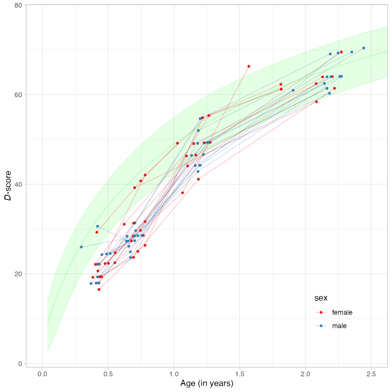
Note that similarity of these curves to growth curves for body height and weight.
The DAZ is an age-standardized D-score with a standard normal distribution with mean 0 and variance 1. We plot the individual DAZ curves relative to the Dutch references by
ggplot(md, aes(x = a, y = daz, group = id, color = factor(sex))) +
  theme_light() +
  theme(legend.position = c(.85, .15)) +
  theme(legend.background = element_blank()) +
  theme(legend.key = element_blank()) +
  scale_color_brewer(palette = "Set1") +
  annotate(
    "rect",
    xmin = -Inf,
    xmax = Inf,
    ymin = -2,
    ymax = 2,
    alpha = 0.1,
    fill = "green"
  ) +
  coord_cartesian(
    xlim = c(0, 2.5),
    ylim = c(-4, 4)
  ) +
  geom_line(lwd = 0.1) +
  geom_point(size = 1) +
  xlab("Age (in years)") +
  ylab("DAZ")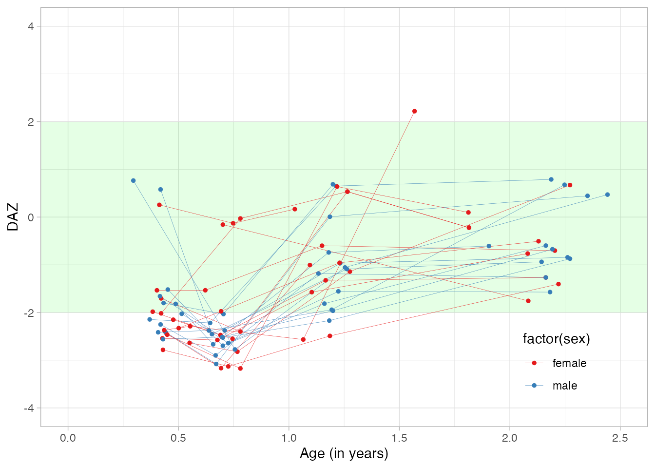
Note that the D-scores and DAZ are a little lower than average. The explanation here is that these all children are born preterm. We can account for prematurity by correcting for gestational age.
The distributions of DAZ for boys and girls show that a large overlap:
ggplot(md) +
  theme_light() +
  scale_fill_brewer(palette = "Set1") +
  geom_density(
    aes(x = daz, group = sex, fill = sex),
    alpha = 0.4,
    adjust = 1.5,
    color = "transparent"
  ) +
  xlab("DAZ")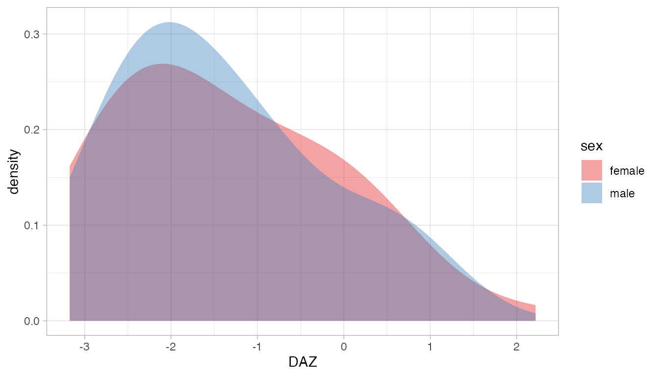
Under the assumption of independence, we may test whether sex differences are constant in age by a linear regression that includes the interaction between age and sex:
##
## Call:
## lm(formula = daz ~ age * sex, data = md)
##
## Residuals:
##      Min       1Q   Median       3Q      Max
## -2.44533 -0.76002 -0.09713  0.65028  3.11002
##
## Coefficients:
##             Estimate Std. Error t value Pr(>|t|)
## (Intercept) -2.13455    0.32499  -6.568 2.62e-09 ***
## age          1.15137    0.27197   4.233 5.27e-05 ***
## sexmale      0.07164    0.45039   0.159    0.874
## age:sexmale -0.12750    0.36137  -0.353    0.725
## ---
## Signif. codes:  0 '***' 0.001 '**' 0.01 '*' 0.05 '.' 0.1 ' ' 1
##
## Residual standard error: 1.137 on 96 degrees of freedom
## Multiple R-squared:  0.2752, Adjusted R-squared:  0.2525
## F-statistic: 12.15 on 3 and 96 DF,  p-value: 8.28e-07
This group of children born very preterm starts around -2.5 SD, followed by a catch-up in child development of approximately 1.0 SD per year. The size of the catch-up is equal for boys and girls.
We may account for the clustering effect by including random intercept and age effects, and rerun as
library(Matrix)
library(lme4, quiet = TRUE)
lmer(daz ~ 1 + age + sex + sex * age + (1 + age | id), data = md)
## Linear mixed model fit by REML ['lmerMod']
## Formula: daz ~ 1 + age + sex + sex * age + (1 + age | id)
## Data: md
## REML criterion at convergence: 304.3713
## Random effects:
## Groups Name Std.Dev. Corr
## id (Intercept) 0.9861
## age 0.6386 -0.85
## Residual 0.9265
## Number of obs: 100, groups: id, 27
## Fixed Effects:
## (Intercept) age sexmale age:sexmale
## -2.1684 1.2067 0.1080 -0.1719This analysis yields the same substantive conclusions as before.