5.3 Estimation of the D-score

The second part of the estimation process is to estimate a D-score. The D-score quantifies the development of a child at a given age. Whereas the instrument developer is responsible for the estimation of item parameters, D-score estimation is more of a task for the user. To calculate the D-score, we need the following ingredients:

• Child’s PASS/FAIL scores on the milestones administered;
• The difficulty estimates of each milestone administered;
• A prior distribution, an estimate of the D-score distribution before seeing any PASS/FAIL score.

Using these inputs, we may use Bayes theorem to calculate the position of the person on the latent variable.

5.3.1 Role of the starting prior

The first two inputs to the D-score will be self-evident. The third component, the prior distribution, is needed to be able to deal with perfect responses. The prior distribution summarizes our knowledge about the D-score before we see any of the child’s PASS/FAIL scores. In general, we like the prior to be non-informative, so that the observed responses and item difficulties entirely determine the value of the D-score. In practice, we cannot use truly non-informative prior because that would leave the D-score for perfect responses (i.e., all PASS or all FAIL) undefined. The choice of the prior is essentially arbitrary, but we can make it in such a way that its impact on the value D-score is negligible, especially for tests where we have more than, say, four items.

Since we know that the D-score depends on age, a logical choice for the prior is to make it dependent on age. In particular, we will define the prior as a normal distribution equal to the expected mean in Figure 4.3 at the child’s age, and with a standard deviation that considerably higher than in Figure 4.3. Numerical example: the mean D-score at the age of 15 months is equal to 53.6\(D\). The standard deviation in Figure 4.3 varies between 2.6\(D\) and 3.0\(D\), with an average of 2.9\(D\). After some experimentation, we found that using a value of 5.0\(D\) for the prior yields a good compromise between non-informativeness and robustness of D-score estimates for perfect patterns. The resulting starting prior for a child aged 15 months is thus \(N(53.6, 5)\).

The reader now probably wonders about a chicken-and-egg problem: To calculate the D-score, we need a prior, and to determine the prior we need the D-score. So how did we calculate the D-scores in Figure 4.3? The answer is that we first took at rougher prior, and calculated two temporary models in succession using the D-scores obtained after solution 1 to inform the prior before solution 2, and so on. It turned out that D-scores in Figure 4.3 hardly changed after two steps, and so there we stopped.

5.3.2 Starting prior: Numerical example

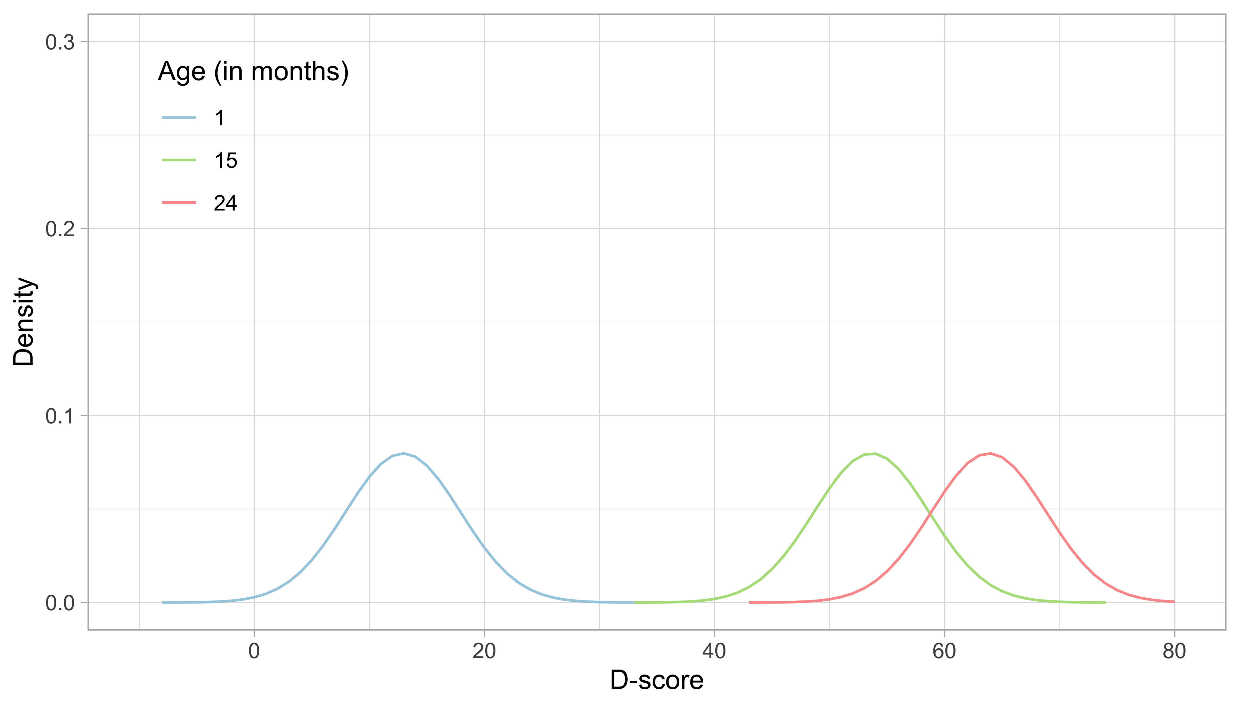
Figure 5.3: Age-dependent starting priors for the D-score at the ages of 1, 15 and 24 months.

Figure 5.3 illustrates starting distributions (priors) chosen according to the principles set above for the ages of 1, 15 and 24 months. As expected, the assumed ability of an infant aged one month is much lower than that of a child aged 15 months, which in turn is lower than the ability of a toddler aged 24 months. The green distribution for 15 months corresponds to the normal distribution \(N(53.6, 5)\).

Another choice that we need to make is the grid of points on which we calculate the prior and posterior distributions. Figure 5.3 uses a grid from -10\(D\) to +80\(D\), with a step size of 1\(D\). These are fixed quadrature points, and there are 91 of them. While these quadrature points are sufficient to estimate D-score for ages up to 2.5 years, it is wise to extend the range for older children with higher D-scores.

5.3.3 EAP algorithm

The algorithm for estimating the D-score is known as the Expected a posteriori (EAP) method, first described by Bock and Mislevy (1982). Calculation of the D-score proceeds item by item. Suppose we have some vague and preliminary idea about the distribution of \(D\), the starting prior (c.f. section 5.3.1), based on age. The procedure uses Bayes rule to update this prior knowledge with data from the first item (using the child’s FAIL/PASS score and the estimated item difficulty) to calculate the posterior. The next step uses this posterior as prior before processing the next item, and so on. The procedure stops when the item pool is exhausted. The order in which items enter does not matter for the result. The D-score is equal to the mean of the posterior calculated after the last question.

5.3.4 EAP algorithm: Numerical example

Suppose we measure two boys aged 15 months, David and Rob, by the DDI. David passes the first four milestones but does not complete the test. Rob completes the test but fails on two out of five items.

Table 5.3 shows the difficulty of each milestone (in the column labelled “Delta”), and the responses of David and Rob for the standard five DDI milestones for the age of 15 months.

The mean D-score for Dutch children aged 15 months is 53.6\(D\), so the milestones are easy to pass at this age, with the most difficult is ddicmm037. David passed all milestones but has no score on the last. Rob fails on ddifmm012 and ddigmm067. How do we calculate the D-score for David and Rob?

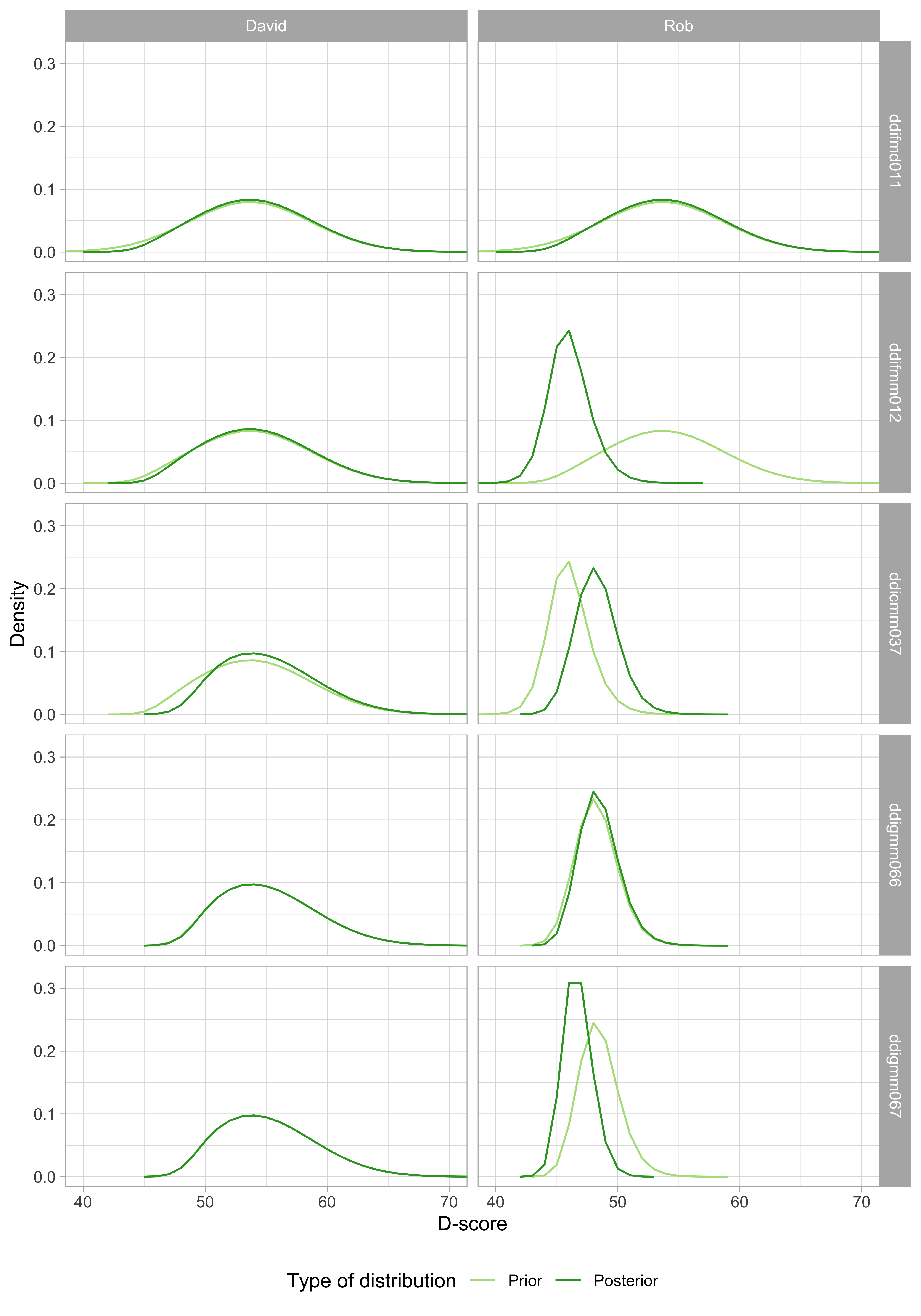
Figure 5.4: D-score distribution for David and Rob before (prior) and after (posterior) a milestone is taken into account.

Figure 5.4 shows how the prior transforms into the posterior after we successively feed the measurements into the calculation. There are five milestones, so the calculation comprises five steps:

1. Both David and Rob pass ddifmd011. The prior (light green) is the same as in Figure 5.3. After a PASS, the posterior will be located more to the right, and will often be more peaked. Both happen here, but the change is small. The reason is that a PASS on this milestone is not very informative. For a child with a true D-score of 53\(D\), the probability of passing ddifmd011 is equal to 0.966. If passing is so common, there is not much information in the measurement.
2. David passes ddifmm012, but Rob does not. Observe that the prior is identical to the posterior of ddifmd011. For David, the posterior is only slightly different from the prior, for the same reason as above. For Rob, we find a considerable change to the left, both for location (from 54.3\(D\) to 47.1\(D\)) and peakedness. This one FAIL lowers Rob’s score by 7.2\(D\).
3. Milestone ddicmm037 is more difficult than the previous two milestones, so a pass on ddicmm037 does have a definite effect on the posterior for both David and Rob.
4. David’s PASS on ddigmm066 does not bring any additional information, so his prior and posterior are virtually indistinguishable. For Rob, we find a slight shift to the right.
5. There is no measurement for David on ddigmm067, so the prior and posterior are equivalent. For Rob, we observe a FAIL, which shifts his posterior to the left.

We calculate the D-score as the mean of the posterior. David’s D-score is equal to 55.7\(D\). Note that the measurement error, as estimated from the variance of the posterior, is relatively large. Rob’s D-score is equal to 47.7\(D\), with a much smaller measurement error. This result is consistent with the design principles of the DDI, which is meant to detect children with developmental delay.

The example illustrates that the quality of the D-score depends on two factors, the match between the true (but unknown) D-score of the child and the difficulty of the milestone.

5.3.5 Technical observations on D-score estimation

• Administration of a too easy set of milestones introduces a ceiling with children that pass all milestones, but whose true D-score could extend well beyond the maximum. Depending on the goal of the measurement, this may or may not be a problem.
• The specification of the prior and posterior distributions requires a set of quadrature points. The quadrature points are taken here as the static and evenly-spaced set of integers between -10 and +80. Using other quadrature points may affect the estimate, especially if the range of the quadrature points does not cover the entire D-score range.
• The actual calculations are here done item by item. A more efficient method is to handle all responses at once. The result will be the same.