4.6 Item response functions

Most measurement models describe the probability of passing an item as a function of the difference between the person’s ability and the item’s difficulty. A person with low ability will almost inevitably fail a heavy item, whereas a highly able person will almost surely pass an easy item.

Let us now introduce a few symbols. We adopt the notation used in Wright and Masters (1982). We use \(\beta_n\) (ability) to refer to the true (but unknown) developmental score of child \(n\). Symbol \(\delta_i\) (difficulty) is the true (but unknown) difficulty of an item \(i\), and \(\pi_{ni}\) is the probability that child \(n\) passes item \(i\). See Appendix A for a complete list.

The difference between the ability of child \(n\) and difficulty of item \(i\) is

\[\beta_n - \delta_i\]

In the special case that \(\beta_n = \delta_i\), the person will have a probability of 0.5 of passing the item.

4.6.1 Logistic model

A widely used method is to express differences on the latent scale in terms of logistic units (or logits) (Berkson 1944). The reason preferring the logistic over the linear unit is that its output returns a probability value that maps to discrete events. In our case, we can describe the probability of passing an item (milestone) as a function of the difference between \(\beta_n\) and \(\delta_i\) expressed in logits.

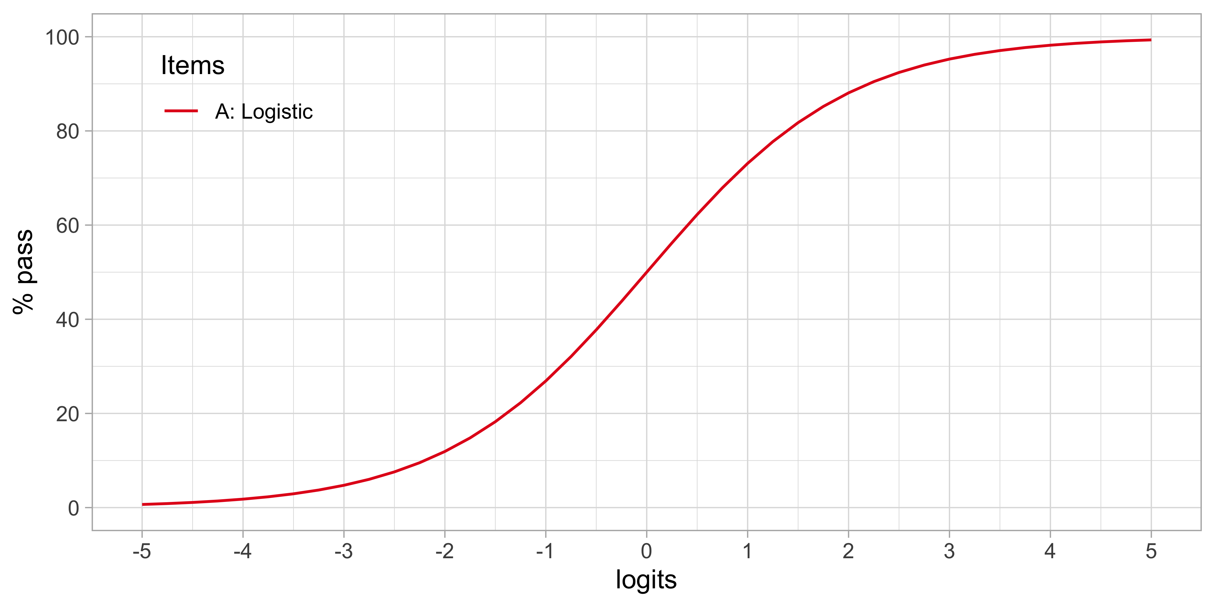
Figure 4.5: Standard logistic curve. Percentage of children passing an item for a given ability-difficulty gap \(\beta_n - \delta_i\).

Figure 4.5 shows how the percentage of children that pass the item varies in terms of the ability-difficulty gap \(\beta_n - \delta_i\). The gap can vary either by \(\beta_n\) or \(\delta_i\) so that we may use the graph in two ways:

• To find the probability of passing items with various difficulties for a child with ability \(\beta_n\). If \(\delta_i = \beta_n\) then \(\pi_{ni} = 0.5\). If \(\delta_i < \beta_n\) then \(\pi_{ni} > 0.5\), and if \(\delta_i > \beta_n\) then \(\pi_{ni} < 0.5\). In words: If the difficulty of the item is equal to the child’s ability, then the child has a 50/50 chance to pass. The child will have a higher than 50/50 chance of passing for items with lower difficulty and have a lower than 50/50 chance of passing for items with difficulties that exceed the child’s ability.
• To find the probability of passing a given item \(\delta_i\) for children that vary in ability. If \(\beta_n < \delta_i\) then \(\pi_{ni} < 0.5\), and if \(\beta_n > \delta_i\) then \(\pi_{ni} > 0.5\). In words: Children with abilities lower than the item’s difficulty will have lower than 50/50 chance of passing, whereas children with abilities that exceed the item’s difficulty will have a higher than 50/50 chance of passing.

Formula (4.1) defines the standard logistic curve:

\[\begin{equation} \pi_{ni} = \frac{\exp(\beta_n - \delta_i)}{1+\exp(\beta_n -\delta_i)} \tag{4.1} \end{equation}\]

One way to interpret the formula is as follows. The logarithm of the odds that a person with ability \(\beta_n\) passes an item of difficulty \(\delta_i\) is equal to the difference \(\beta_n-\delta_i\) (Wright and Masters 1982). For example, suppose that the probability that person \(n\) passes milestone \(i\) is \(\pi_{ni} = 0.5\). In that case, the odds of passing is equal to \(0.5 / (1-0.5) = 1\), so \(\log(1) = 0\) and thus \(\beta_n = \delta_i\). If \(\beta_n - \delta_i = \log(2) = 0.693\) person \(n\) is two times more likely to pass than to fail. Likewise, if the difference is \(\beta_n - \delta_i = \log(3) = 1.1\), then person \(n\) is three more likely to pass. And so on.

4.6.2 Types of item response functions

The standard logistic function is by no means the only option to map the relationship between the latent variable and the probability of passing an item. The logistic function is the dominant choice in IRT, but it is instructive to study some other mappings. The item response function maps success probability against ability.

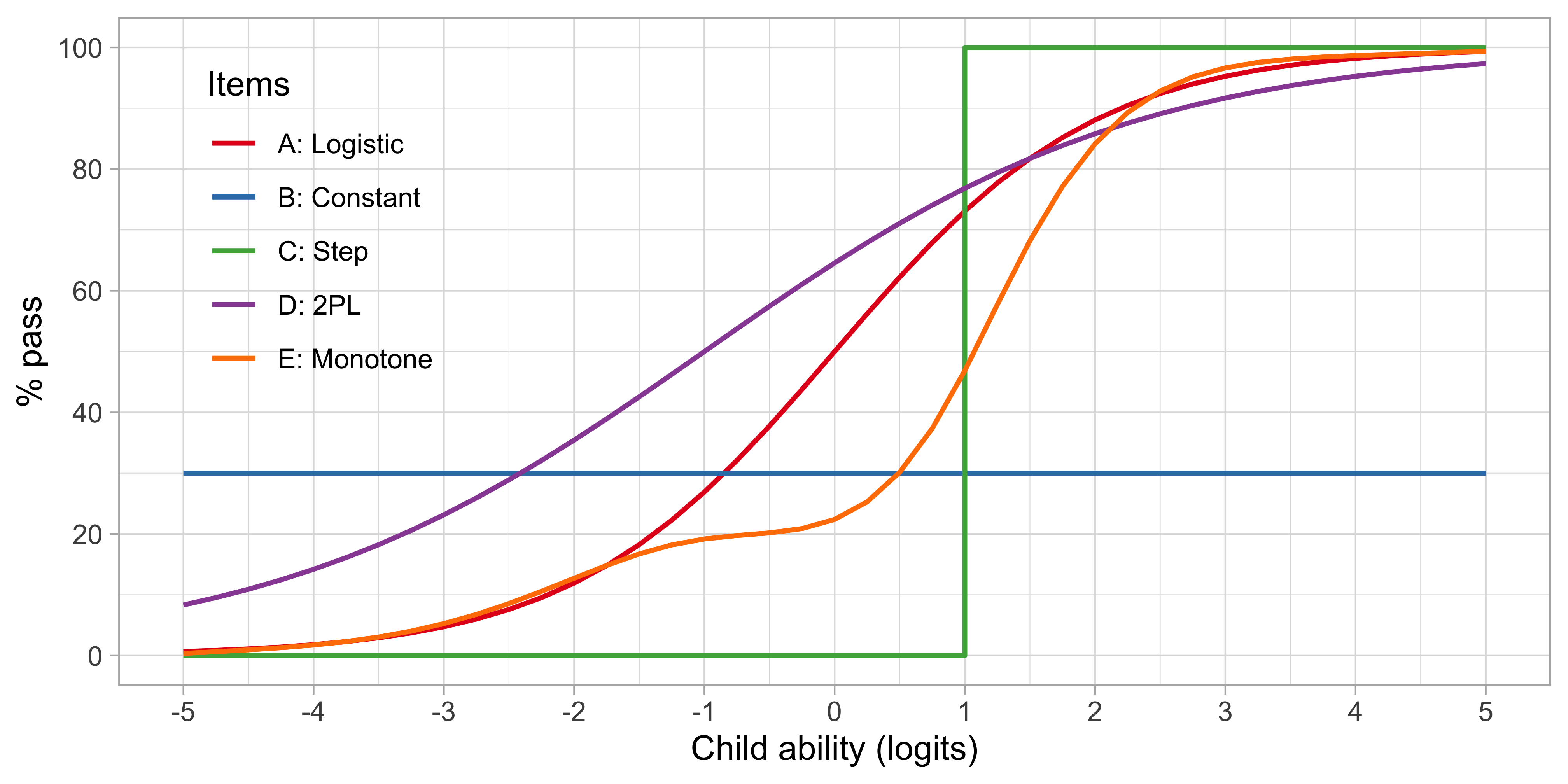
Figure 4.6: Item response functions for five hypothetical items, each demonstrating a positive relation between ability and probability to pass.

Figure 4.6 illustrates several other possibilities. Let us consider five hypothetical items, A-E. Note that the horizontal axis now refers to the ability, instead of the ability-item gap in 4.5.

• A: Item A is the logistic function discussed in Section 4.6.
• B: For item B, the probability of passing is constant at 30 per cent. This 30 per cent is not related to ability. Item B does not measure ability, only adds to the noise, and is of low quality.
• C: Item C is a step function centred at an ability level of 1, so all children with an ability below 1 logit fail and all children with ability above 1 logit pass. Item C is the ideal item for discriminating children with abilities above and below 1. The item is not sensitive to differences at other ability levels, and often not so realistic in practice.
• D: Like A, item D is a smoothly increasing logistic function, but it has an extra parameter that allows it to vary its slope (or discrimination). The extra parameter can make the curve steeper (more discriminatory) than the red curve, in the limit approaching a step curve. It can also become shallower (less discriminatory) than the red curve (as plotted here), in the limit approaching a constant curve (item B). Thus, item D generalizes items A, B or C.
• E: Item E is even more general in the sense that it need not be logistic, but a general monotonically increasing function. As plotted, the item is insensitive to abilities between -1 and 0 logits, and more sensitive to abilities between 0 to 2 logits.

These are just some examples of how the relationship between the child’s ability and passing probability could look. In practice, the curves need not start at 0 per cent or end at 100 per cent. They could also be U-shaped, or have other non-monotonic forms. See Coombs (1964) for a thorough overview of such models. In practice, most models are restricted to shapes A-D.

4.6.3 Person response functions

We can reverse the roles of persons and items. The person response function tells us how likely it is that a single person can pass an item, or more commonly, a set of items.

Let us continue with items A, C and D from Figure 4.6, and calculate the response function for three children, respectively with abilities \(\beta_1 = -2\), \(\beta_2 = 0\) and \(\beta_3 = 2\).

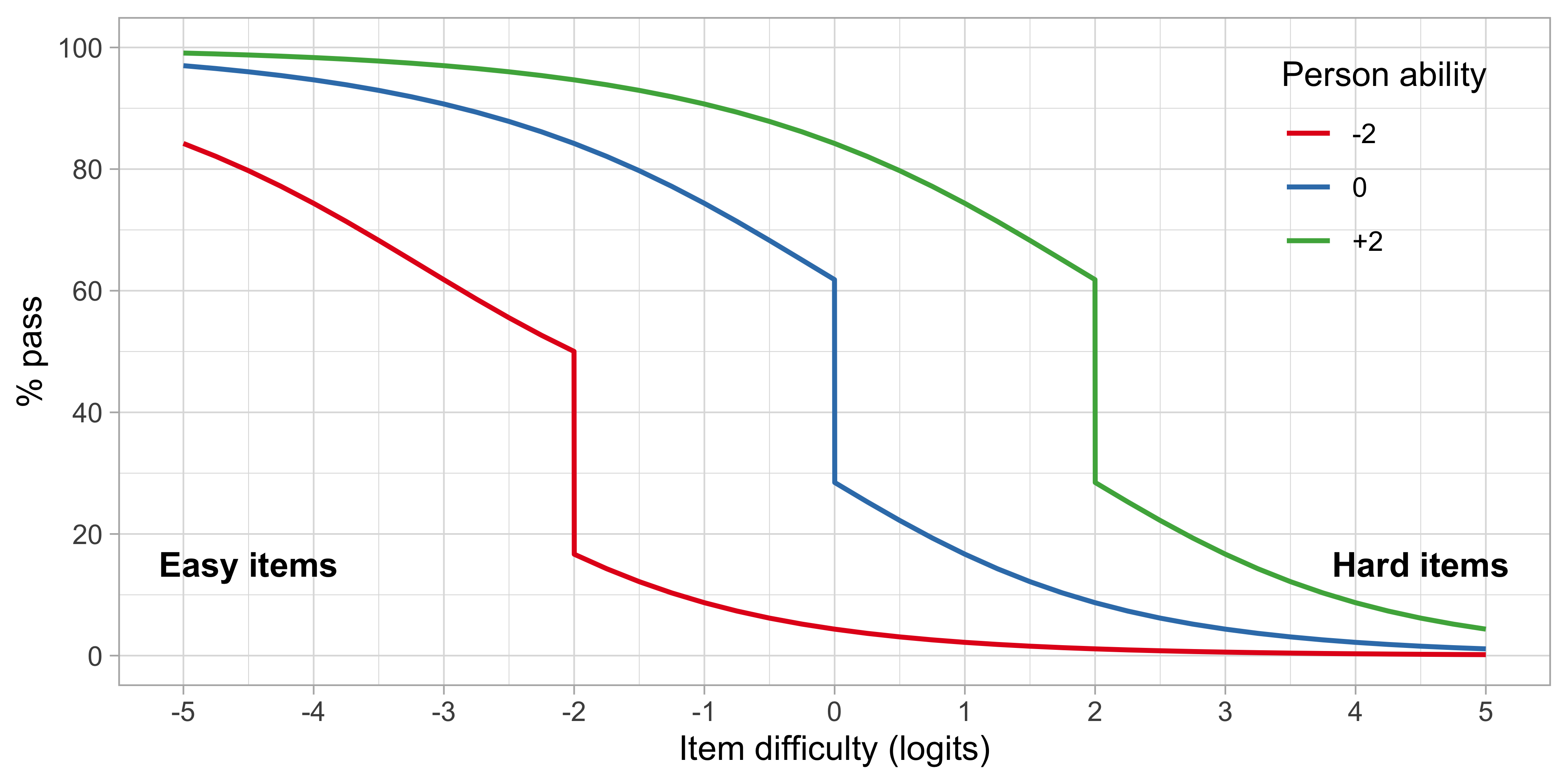
Figure 4.7: Person response functions for three children with abilities -2, 0 and +2, using a small test of items A, C and D.

Figure 4.7 presents the person response functions from three persons with abilities of -2, 0 and +2 logits. We calculate the functions as the average of response probabilities on items A, C and D. Thus, on average, we expect that child 1 logit will pass an easy item of difficulty -3 in about 60 per cent of the time, whereas for an intermediate item of difficulty of -1 the passing probability would be 10 per cent. For child 3, with higher ability, these probabilities are quite different: 97% and 90%. The substantial drop in the middle of the curve is due to the step function of item A.