6.1 Item fit
The philosophy of the Rasch model is different from conventional statistical modelling. It is not the task of the Rasch model to account for the data. Rather it is the task of the data to fit the Rasch model. We saw this distinction before in Section 4.5.2.
The goal of model-fit assessment is to explore and quantify how well empirical data meet the requirements of the Rasch model. One way to gauge model-fit is to compare the observed probability of passing an item to the fitted item response curve for endorsing the item.
The fitted item response curve for each item \(i\) is modeled as:
\[P_{ni} = \frac{\exp(\hat\beta_{n} - \hat\delta_{i})}{1+\exp(\hat\beta_{n}-\hat\delta_{i})},\]
where \(\hat\beta_n\) is the estimated ability of child \(n\) (the child’s D-score), and where \(\hat\delta_i\) is the estimated difficulty of item \(i\). This is equivalent to formula (4.1) with the parameters replaced by estimates. Section 5 described process of parameter estimation in some detail.
6.1.1 Well-fitting item response curves
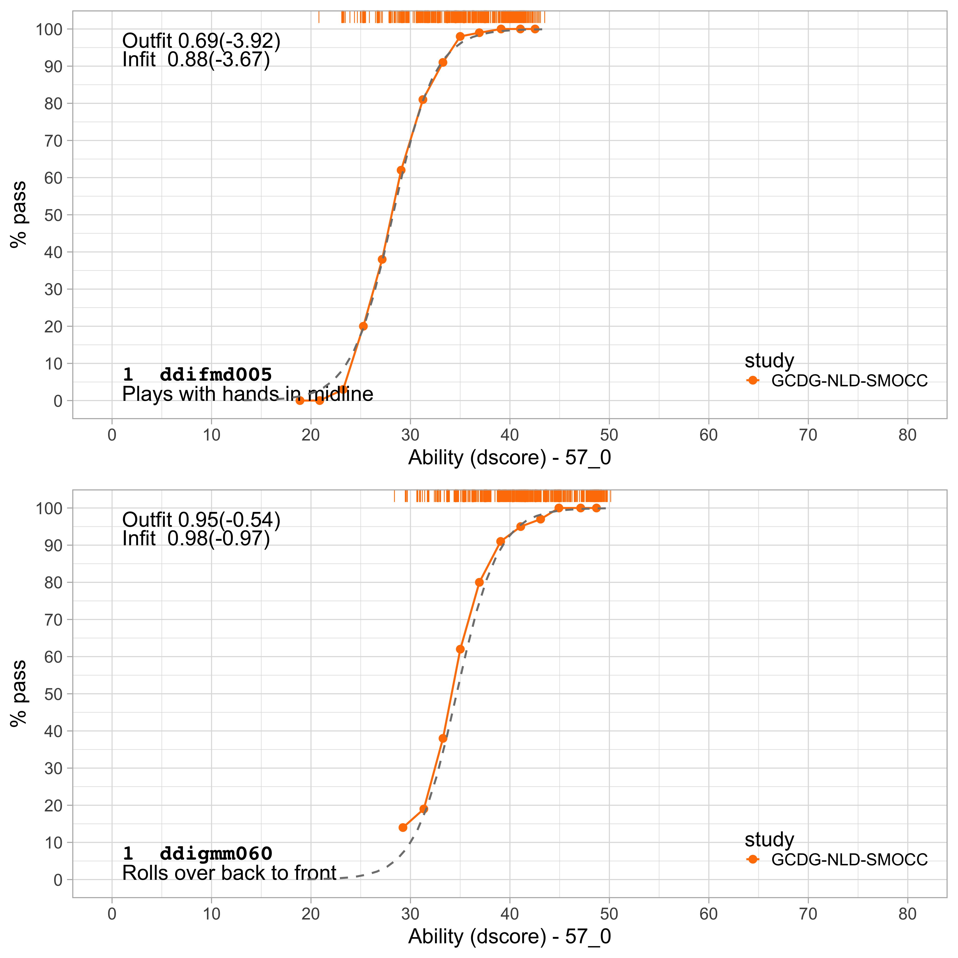
Figure 6.1: Empirical and fitted item response curves for two milestones from the DDI (SMOCC data).
The study of item fit involves comparing the empirical and fitted probabilities at various levels of ability. Figure 6.1 shows the item characteristics curves of two DDI milestones. The orange line represents the empirical probability at different ability levels. The dashed line represents the estimated item response curve according to the Rasch model. The observed and estimated curves are close together, so both items fit the model very well.
6.1.2 Item response curves showing severe underfit
There are many cases where things are less bright.
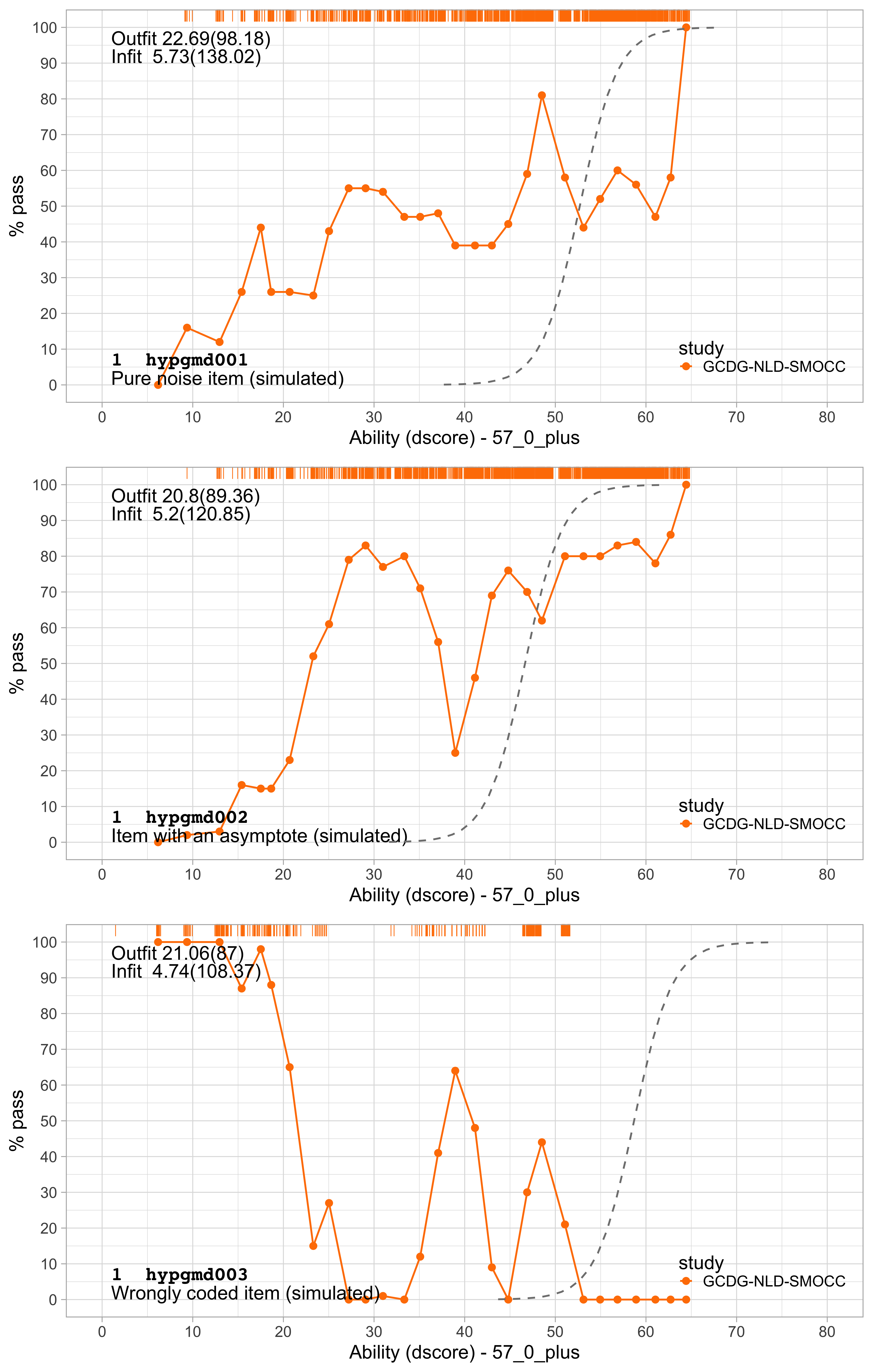
Figure 6.2: Three simulated items that illustrate various forms of item misfit.
Figure 6.2 shows three forms of severe underfit from three artificial items. These items were simulated to have a low fit, added to the DDI, and we estimated their parameters by the methods of Section 5. For the first item, hypgmd001, the probability of passing is almost constant across ability, so retaining this item essentially only adds to the noise. Item hypgmd002 converges to an asymptote around 80 per cent and has a severe dip in the middle. The strong relation to age causes the drop. Item hypgmd003 appears to have the wrong coding. Also, we often see the spike-like behaviour in the middle when two or more different items erroneously share identical names.
Removal of items with a low fit can substantially improve overall model fit.
6.1.3 Item response curves showing overfit
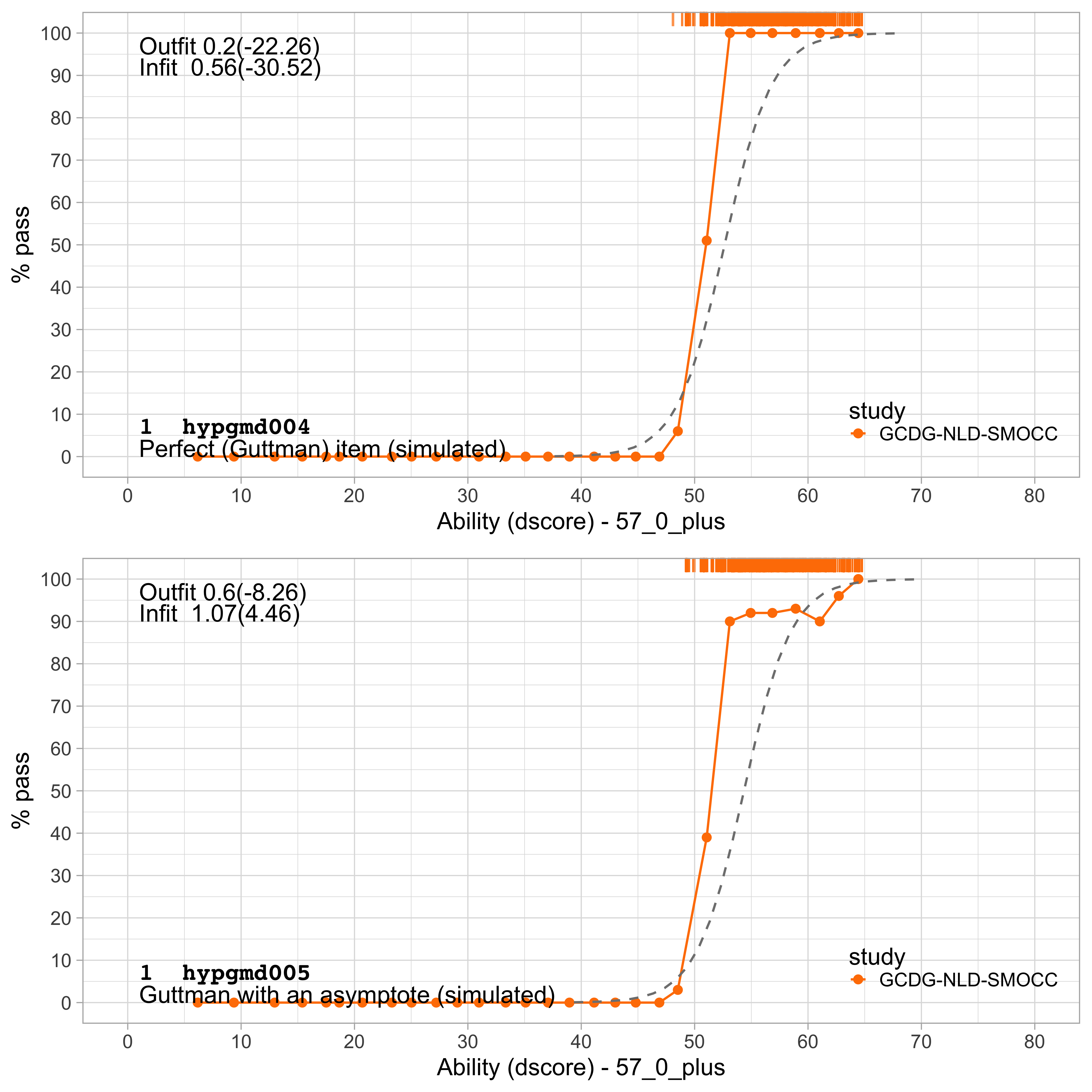
Figure 6.3: Two simulated items that illustrate item overfit.
Figure 6.3 shows two artificial items with two forms of overfitting. The curve of item hypgmd004 is much steeper than the modelled curve. Thus, just this one item is exceptionally well-suited to distinguish children with a D-score below 50\(D\) from those with a score above 50\(D\). Note that the item isn’t sensitive anywhere else on the scale. In general, having items like these is good news, because they allow us to increase the reliability of the instrument. One should make sure, though, that FAIL and PASS scores are all measured (not imputed) values.
Multiple perfect items could hint to a violation of the local independence assumption (c.f. Section 4.5). Developmental milestones sometimes have combinations of responses that are impossible. For example, one cannot walk without being able to stand, so we will not observe the inconsistent combination (stand: FAIL, walk: PASS). This impossibility leads to more consistent responses that would be expected by chance alone. In principle, one could combine the two such items into one three-category item, which effectively set the probability of inconsistent combinations to zero.
Item hypgmd005 is also steep, but has an asymptote around 80 per cent. This tail behaviour causes discrepancies between the empirical and modeled curves around the middle of the probability scale. In general, we may remove such items if a sufficient number of alternatives is available.
6.1.4 Item infit and outfit
We quantify item fit by item infit and outfit. Both are aggregates of the model residuals. The observed response \(x_{ni}\) of person \(n\) on item \(i\) can be \(0\) or \(1\).
The standardized residual \(z_{ni}\) is the difference between the observed response \(x_{ni}\) and the expected response \(P_{ni}\), divided by the expected binomial standard deviation,
\[z_{ni} = \frac{x_{ni}-P_{ni}}{\sqrt{W_{ni}}},\]
where the expected response variance \(W_{ni}\) is calculated as
\[W_{ni} = P_{ni}(1-P_{ni}).\]
Item infit is the total of the squared residuals divided by the sum of the expected response variances \(W_{ni}\)
\[\mathrm{Item\ infit} = \frac{\sum_{n}^N (x_{ni}-P_{ni})^2}{\sum_n^N W_{ni}}.\]
Item outfit is calculated as the average (over \(N\) measurements) of the squared standardized residual
\[\mathrm{Item\ outfit} = \frac{\sum_{n}^N z_{ni}^2}{N}.\]
The expected value of both infit and outfit is equal to 1.0. The interpretation is as follows:
- If infit and outfit are 1.0, then the item perfectly fits the Rasch model, as in Figure 6.1;
- If infit and outfit > 1.0, then the item is not fitting well. The amount of underfit is quantified by infit and outfit, as in 6.2;
- If infit and outfit < 1.0, then the item fits the model better than expected (overfit). Overfitting is quantified by infit and outfit, as in 6.3.
Infit is more sensitive to disparities in the middle of the probability scale, whereas outfit is the better measure for discrepancies at probabilities close to 0 or 1. Lack of fit is generally easier to spot at the extremes. The two measures are highly correlated. Achieving good infit is more valuable than a high outfit.
Values near 1.0 are desirable. There is no cut and dried cut-off value for infit and outfit. In general, we want to remove underfitting items with infit or outfit values higher than, say, 1.3. Overfitting items (with values lower than 1.0) are not harmful. Preserving these items may help to increase the reliability of the scale. The cut-off chosen also depends on the number of available items. When there are many items to choose from, we could use a stricter criterion, say infit and outfit < 1.0 to select only the absolute best items.
6.1.5 Infit and outfit in the DDI
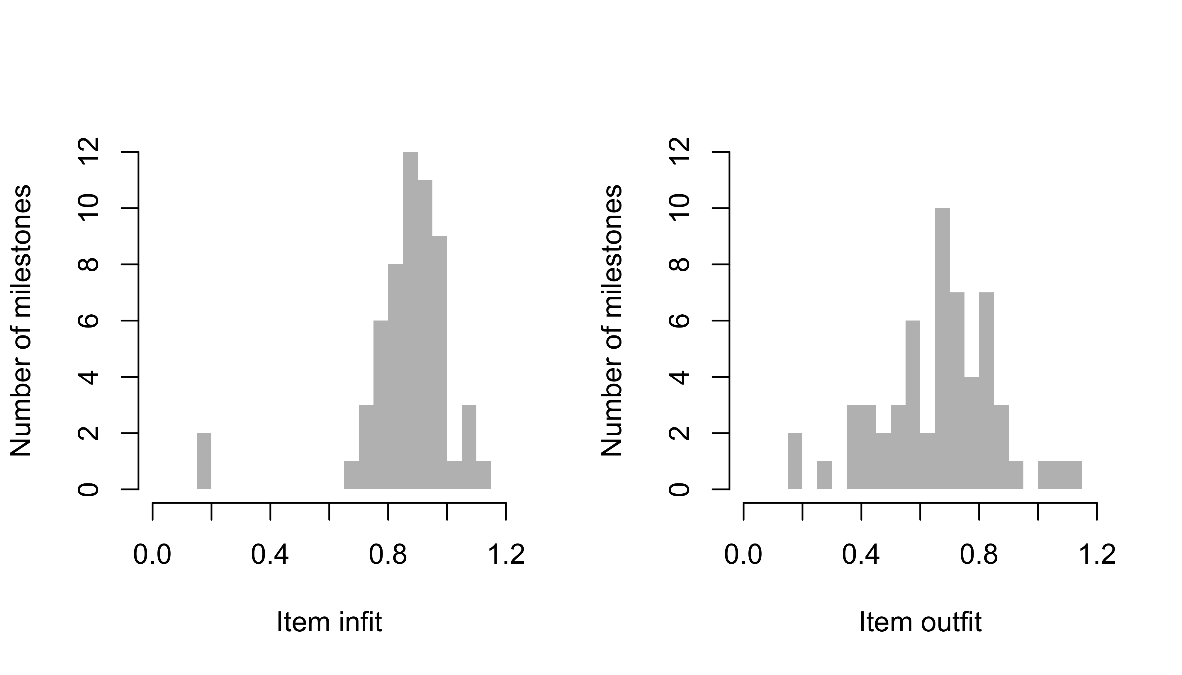
Figure 6.4: Frequency distribution of infit (left) and outfit (right) of 57 milestones from the DDI (SMOCC data).
Figure 6.4 displays the histogram of the 57 milestones from the DDI (c.f. Section 4.1). Most infit values are within the range 0.6 - 1.1, thus indicating excellent fit. The two milestones with shallow infit values are ddigmd052 and ddigmd053. These two items screen for paralysis for newborns, so the data contain hardly any fails on these milestones. The outfit statistics also indicate a good fit.